What Is a Vector Database?
|
This content was generated with the assistance of AI and should be verified against the official documentation of each tool and framework before being relied on in production. This section’s bibliography lists the reference material consulted while preparing these pages. |
The code on this page targets Python 3.12 with NumPy, and PostgreSQL 17 with pgvector 0.8.6 for the SQL examples. It introduces the vocabulary — similarity, nearest neighbour, the vector data type, and the hybrid architecture of vector component plus metadata component plus integration layer — that the rest of this section builds on.
Why unstructured data needs semantic search
Keyword search matches the literal words in a query against the literal words in a document. That works well for structured data and exact identifiers, but it breaks down on the kind of language people actually use when they ask questions.
Say a customer types "get my money back" into a support search box, but every article in the knowledge base is
titled "Refund Policy" or "How to Request a Refund". A keyword index built on money, back, get finds
nothing useful: none of those words appear in the relevant article, even though the intent is identical. The
same failure shows up in reverse. A user searching "laptop won’t turn on" gets no hits from an article titled
"Troubleshooting Power and Boot Issues", because "laptop", "turn" and "on" never appear together in that text
either. Keyword search needs the same words; semantic search needs the same meaning.
Semantic search fixes this by comparing meaning instead of vocabulary. An embedding model maps a stretch of text to a vector — a fixed-length array of floating-point numbers — such that texts with similar meaning end up as vectors that are close together in that space, regardless of which words were used to express them. "Get my money back" and "How to request a refund" land near each other; "laptop won’t turn on" lands near "troubleshooting power and boot issues" even though the two share no words at all.
Keyword matching still has a role precisely where semantic search struggles: on ambiguous words. The word "apple" refers to a fruit in one document and to a technology company in another; a keyword index treats both occurrences identically, and a naive embedding of the bare word "apple" in isolation is similarly underdetermined. Embeddings resolve this ambiguity only once the word sits in a sentence — "apple pie recipe" and "Apple’s quarterly earnings" embed far apart, because the model conditions the vector on surrounding context. This is why hybrid search (combining keyword and vector signals) is common in practice, and why retrieval quality depends on embedding whole passages rather than isolated terms; both points are covered on Hybrid Search & Re-ranking.
Consider the DocsAssistant agent used throughout this section: an AI agent that answers questions about a
corpus of technical documentation such as this site’s own AsciiDoc pages. A user asks DocsAssistant, "how do I
speed up similarity search?" The corpus contains a page titled "HNSW indexes" (docs/vector-rag/hnsw.adoc)
that never uses the phrase "speed up similarity search" verbatim — it talks about approximate nearest-neighbour
graphs, ef_search, and recall/latency trade-offs. A keyword search over that corpus, built on the literal
query terms, would rank the HNSW page low or miss it entirely. A semantic search embeds the query and the
page’s chunks with the same model and ranks by vector closeness, so "speed up similarity search" lands close to
a chunk explaining that raising ef_search trades latency for recall in an HNSW index — exactly the
"HNSW indexes" chunk DocsAssistant should surface. This mermaid diagram contrasts the two paths for that same
query:
The vector data type and its three operations
A vector database’s core data type is the embedding vector: a fixed-length, dense array of floating-point numbers produced by an embedding model, typically hundreds to a few thousand dimensions. Everything the engine does reduces to three operations on that data type.
-
Similarity — a scalar score (or its inverse, a distance) between two vectors that quantifies how close their meanings are. Similarity Metrics & Semantic Search covers the metrics (cosine, L2, inner product) and when each applies.
-
(Approximate) nearest neighbour — given a query vector, find the
kvectors in a collection with the highest similarity (lowest distance). Doing this exactly means comparing the query to every stored vector; at scale, engines trade a small amount of accuracy for speed with an approximate nearest-neighbour (ANN) index such as HNSW or IVF, covered in ANN Indexes: Flat, IVF, HNSW and Beyond. -
Vector arithmetic — vectors support addition, subtraction and scaling like any other numeric vector, and in a well-trained embedding space these operations track semantic relationships (the classic "king minus man plus woman equals queen" example). Embeddings demonstrates this with a runnable Word2Vec example; centroids computed by averaging vectors are also used for clustering and for representing a whole document from its chunk vectors.
The following NumPy snippet performs brute-force nearest-neighbour search: it embeds five toy 4-dimensional "vectors" by hand (standing in for real embeddings), computes cosine similarity between a query vector and each of them, and returns the closest match. This is exact nearest-neighbour search — the same operation an ANN index approximates at scale — and is exactly what Similarity Metrics & Semantic Search does later at DocsAssistant scale.
import numpy as np

# Five toy 4-D vectors standing in for real embeddings (which would be
# hundreds or thousands of dimensions, produced by an embedding model).
vectors = np.array([
    [0.9, 0.1, 0.0, 0.1],   # "refund policy"
    [0.8, 0.3, 0.1, 0.0],   # "how to request a refund"
    [0.1, 0.9, 0.2, 0.0],   # "laptop troubleshooting"
    [0.0, 0.1, 0.9, 0.2],   # "fruit and nutrition"
    [0.2, 0.0, 0.8, 0.3],   # "apple pie recipe"
])
labels = [
    "refund policy",
    "how to request a refund",
    "laptop troubleshooting",
    "fruit and nutrition",
    "apple pie recipe",
]

query = np.array([0.85, 0.2, 0.05, 0.05])  # "get my money back"


def cosine_similarity(a: np.ndarray, b: np.ndarray) -> np.ndarray:
    a_norm = a / np.linalg.norm(a, axis=-1, keepdims=True)
    b_norm = b / np.linalg.norm(b)
    return a_norm @ b_norm


scores = cosine_similarity(vectors, query)
order = np.argsort(-scores)  # descending: most similar first

for rank, idx in enumerate(order, start=1):
    print(f"{rank}. {labels[idx]!r} (cosine similarity={scores[idx]:.3f})")
Running this prints "how to request a refund" and "refund policy" as the top two matches for the query "get my
money back", even though none of the query’s words appear in either label — the brute-force scan over
cosine_similarity is doing exactly the semantic match described above. See the
NumPy linalg.norm documentation for
the norm used to normalise vectors before the dot product.
Use cases
Because similarity and nearest-neighbour search generalise past exact text matching, the same vector database primitives support several distinct workloads:
-
Semantic search — finding documents, products or support articles by meaning rather than keyword overlap, as in the "get my money back" example above.
-
Retrieval-augmented generation (RAG) — fetching the passages most relevant to a prompt so an LLM can ground its answer in retrieved context instead of relying only on parameters learned at training time; see RAG Fundamentals.
-
Recommendations — "more like this" by finding items whose embeddings are close to a user’s history or to a seed item.
-
Deduplication and near-duplicate detection — flagging records whose embeddings sit within a small distance of each other, catching paraphrases or reformattings that an exact-match or hash comparison would miss.
-
Anomaly detection — treating points that are far from every cluster of "normal" embeddings as outliers, useful for fraud signals or malformed records.
-
Multimodal retrieval — embedding images, audio or text into a shared vector space (for example with CLIP, covered in Embeddings) so a text query can retrieve images, or vice versa.
database/choosing-the-right-database.adoc#_vector_databases introduces the same use-case list from the angle of choosing a database category; this page and the rest of this section go into the mechanics behind it.
SQL FLOAT[] vs. vector-specific capabilities
It is tempting to store an embedding in an ordinary relational column and call it a day:
-- Works for storage, but has no vector-aware behaviour at all.
CREATE TABLE chunk_embeddings_naive (
    chunk_id   bigint PRIMARY KEY,
    embedding  FLOAT[]   -- just an array of floats
);
This compiles and stores the data, but a plain FLOAT[] column is opaque to the database: there is no
ORDER BY clause that means "closest to this vector", no operator for cosine or Euclidean distance, and no
index type that can avoid a full table scan to answer a nearest-neighbour query. Every similarity search
against chunk_embeddings_naive means fetching every row into application code and computing distances there — exactly what the NumPy example above does for five rows, but unworkable once the table holds millions.
A vector-specific extension such as pgvector adds a real vector type, distance operators, and ANN index types that make PostgreSQL itself capable of answering the query efficiently:
CREATE EXTENSION IF NOT EXISTS vector;

CREATE TABLE chunk_embeddings (
    chunk_id   bigint PRIMARY KEY REFERENCES chunks (id) ON DELETE CASCADE,
    model      text NOT NULL,
    embedding  vector(768)  -- fixed dimensionality, enforced by the type
);

CREATE INDEX chunk_embeddings_hnsw
    ON chunk_embeddings
    USING hnsw (embedding vector_cosine_ops)
    WITH (m = 16, ef_construction = 64);

SELECT chunk_id, embedding <=> $1 AS distance
FROM chunk_embeddings
ORDER BY embedding <=> $1
LIMIT 5;
The vector(768) column enforces dimensionality at write time, the <⇒ operator computes cosine distance
directly in SQL, and the hnsw index lets PostgreSQL answer ORDER BY embedding <⇒ $1 LIMIT 5 without
scanning the whole table. PostgreSQL & pgvector covers pgvector’s full type and
operator set; ANN Indexes: Flat, IVF, HNSW and Beyond covers how the HNSW index itself works. See the
pgvector README for the authoritative type and operator reference.
NoSQL with vector extensions sits between the two: document and key-value stores such as MongoDB, Couchbase, Redis and Neo4j have added native vector indexes on top of their existing storage engine. This is enough when the workload is already a good fit for that database (documents already model the domain well, or the team already operates that engine) and vector search is one feature among several — filtering, transactions, graph traversal — that the same data needs. Because the vector index is retrofitted onto a general-purpose engine, it typically supports fewer distance metrics, quantization options or ANN algorithm choices than a database built around vectors from the start, and very large vector workloads can compete with the engine’s other responsibilities for memory and I/O. See Text, wildcard, geospatial & Atlas search, Full-Text & Vector Search, Analytics & Eventing, Vector Search: Query Engine & Vector Sets and Vector Search and GenAI for how each one implements it.
Purpose-built vector engines (Qdrant, Milvus, Weaviate and similar) invert that trade-off: vector search is the primary workload the storage engine, index build path and query planner are designed around, which usually means more ANN algorithm and quantization choices, and horizontal scaling built for billions of vectors, at the cost of running (or paying for) a separate system alongside whatever stores the rest of the data. See Qdrant Reference and The Vector Database Landscape for how the categories compare.
The hybrid architecture
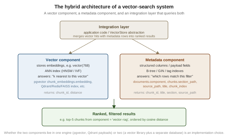
Whichever category a vector database falls into, it is answering two different kinds of question at once: "which vectors are closest to this one" and "which rows satisfy this filter" — and a real query usually needs both together ("closest chunks where `component = 'vector-rag'`"). Every engine, in effect, implements three cooperating pieces:
-
A vector component that stores embeddings and answers nearest-neighbour queries via an ANN index.
-
A metadata component that stores structured fields (titles, tags, timestamps, tenant IDs) and answers filter queries via ordinary indexes (B-tree, GIN, tag indexes).
-
An integration layer that accepts a single logical query, dispatches the vector and filter parts to the right component, and merges the results into one ranked, filtered answer.
In pgvector, all three pieces live inside PostgreSQL itself: the vector column and its HNSW index are the
vector component, ordinary columns and their B-tree/GIN indexes are the metadata component, and the query
planner is the integration layer. In an engine like Qdrant, the vector component is the collection’s HNSW
index and the metadata component is its payload index, but the same three-part shape holds. LangChain’s and
Spring AI’s VectorStore abstractions, described below, are an integration layer implemented in application
code rather than inside the database engine.
An informal hybrid query against DocsAssistant’s corpus — "the 5 chunks most similar to this query vector,
restricted to the vector-rag component" — reads naturally as a sentence, but the integration layer has to
turn it into a single query plan that touches both components. In pgvector, that same request is one ordinary
SQL statement, because both components live in the same engine:
-- Informal: "5 chunks closest to $1, but only from the vector-rag component"
SELECT c.id, c.content, ce.embedding <=> $1 AS distance
FROM chunk_embeddings ce
JOIN chunks c ON c.id = ce.chunk_id
JOIN documents d ON d.id = c.document_id
WHERE d.component = 'vector-rag'   -- metadata component: B-tree filter
ORDER BY ce.embedding <=> $1       -- vector component: HNSW-backed ANN order
LIMIT 5;
The WHERE d.component = 'vector-rag' clause is answered by the B-tree index on documents(component) (the
metadata component); the ORDER BY … LIMIT 5 clause is answered by the HNSW index on chunk_embeddings
(the vector component); PostgreSQL’s planner is the integration layer that decides how to combine them
efficiently. Metadata Filtering covers what can go wrong when the filter and
the ANN index interact naively (the overfetch-then-filter failure mode) and how pgvector’s iterative index
scans address it.
In LangChain and Spring AI
Both frameworks expose the "integration layer" of the hybrid architecture above as a single abstraction, so application code issues one call and the abstraction dispatches to whichever vector and metadata components the underlying store actually has.
LangChain
LangChain’s VectorStore interface is exactly this integration layer: similarity_search takes a
natural-language query plus a metadata filter, embeds the query, and returns documents already merged with
their metadata — the caller never issues a separate vector query and a separate filter query. This is the
same "5 closest chunks from the vector-rag component" request as the SQL above:
from langchain_ollama import OllamaEmbeddings
from langchain_postgres import PGVector

vector_store = PGVector(
    embeddings=OllamaEmbeddings(model="nomic-embed-text"),
    collection_name="docsassistant",
    connection="postgresql+psycopg://docs:docs@localhost:5432/docsassistant",
    use_jsonb=True,
)
docs = vector_store.similarity_search(
    "search_query: how do I speed up similarity search",
    k=5,
    filter={"component": {"$eq": "vector-rag"}},  # metadata component
)
for doc in docs:
    print(doc.metadata["source_path"], doc.page_content[:60])
See the official LangChain PGVector
page. Concrete stores such as PGVector or Qdrant implement the interface against pgvector’s or Qdrant’s
own vector and metadata components; see
Integrating with LangChain — Vector stores for the store-by-store detail.
Spring AI
Spring AI’s VectorStore interface plays the same role: one similaritySearch call combines the vector
similarity search and the metadata filter, regardless of whether the backing store is PgVectorStore, Redis,
or another implementation:
List<Document> docs = vectorStore.similaritySearch(
    SearchRequest.builder()
        .query("how do I speed up similarity search")
        .topK(5)
        .filterExpression("component == 'vector-rag'")  // metadata component
        .build());

docs.forEach(doc -> System.out.println(doc.getMetadata().get("source_path") + " " + doc.getScore()));
See the official Spring AI Vector Databases
page, and Integrating with
Spring AI — The VectorStore API for configuration and usage detail.
Related pages
-
Embeddings — how embedding models produce the vectors this page treats as a given data type.
-
Similarity Metrics & Semantic Search — the similarity metrics behind the NumPy example above, at DocsAssistant scale.
-
ANN Indexes: Flat, IVF, HNSW and Beyond — how HNSW and IVF approximate the nearest-neighbour operation.
-
PostgreSQL & pgvector — the full pgvector type and operator reference used above.
-
database/choosing-the-right-database.adoc#_vector_databases — choosing a vector database category for a given workload.
-
Qdrant Reference — a purpose-built vector engine reference.
-
Vector Search: Query Engine & Vector Sets — a NoSQL-with-extensions vector search implementation.