Similarity Metrics & Semantic Search
|
This content was generated with the assistance of AI and should be verified against the official documentation of each tool and framework before being relied on in production. This section’s bibliography lists the reference material consulted while preparing these pages. |
Examples on this page use Python 3.12 and NumPy, and are checked against pgvector 0.8.6, FAISS 1.15.1 and sqlite-vec 0.1.9 where an engine-specific detail is shown. Every ANN index and every vector database ultimately ranks candidates with one of a small set of distance or similarity functions. Picking the right one — and matching it consistently between the index that was built and the query that searches it — is one of the most common sources of silently wrong results in a vector-database deployment.
The metrics
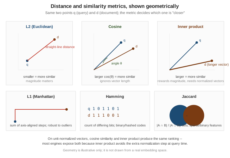
Squared L2 drops the square root ( ); it preserves the same ranking as L2 while avoiding a square-root computation per candidate, which is why most engines default to it internally even when they report plain L2 to the caller.
Inner product (dot product) depends on both the angle between two vectors and their magnitudes. It is the right metric when a model’s documentation says its raw, unnormalized outputs are meant to be compared by dot product (the vector’s length then carries signal, as with learned sparse models such as SPLADE), or when the vectors are already unit-normalized, where it gives the same ranking as cosine (see below). Used carelessly on unnormalized vectors from a cosine-trained model, it can rank a longer, less relevant vector above a shorter, more relevant one.
Cosine similarity is the inner product divided by both vectors' norms, so it measures the angle between
two vectors and ignores their length entirely. It is the default for most sentence-embedding models,
including the Ollama nomic-embed-text model the DocsAssistant scenario uses throughout this section: its
search_document: ` / `search_query: ` task prefixes make the model asymmetric (questions and passages are
embedded differently), but the resulting vectors are still compared by cosine, which is why every DocsAssistant
index uses `vector_cosine_ops
(or inner product over normalized vectors).
L1 (Manhattan/taxicab distance) sums absolute per-dimension differences instead of squaring them, which makes it less sensitive to a single dimension with an unusually large difference (an outlier feature) than L2. It shows up more often on sparse or count-like feature vectors than on dense neural embeddings.
Hamming distance counts differing positions between two equal-length bit strings. It only makes sense on binary vectors — the output of binary quantization, a locality-sensitive hash, or a natively binary embedding model — because it needs single-bit comparisons to be cheap, which is what makes it attractive for that case: see Quantization & Compression for how binary codes are produced.
Jaccard similarity treats each vector as a set (or a sparse vector as the set of its non-zero positions) and compares set overlap rather than coordinate-wise distance. It is common on sparse/keyword-style representations and on categorical feature sets, and it is unrelated to the geometric metrics above — there is no vector space it is computing a distance "in".
Selection heuristics
-
Cosine is the safe default for dense text embeddings from a modern sentence-embedding model, because those models are trained (or explicitly normalized) so that direction, not magnitude, carries the meaning.
-
Inner product is faster to compute (no division, no square root) and is the right choice when the vectors are already unit-normalized — see the equivalence below — or when the embedding model is specifically trained for it (its model card says to compare raw outputs by dot product, so magnitude is meaningful).
-
L2 / squared L2 fits image and audio embeddings and classical clustering pipelines (k-means is defined in terms of squared L2), and any space where absolute distance, not just direction, is meaningful.
-
L1 is a reasonable alternative to L2 when the data is expected to have outlier dimensions and a more robust, less quadratically-penalized distance is wanted.
-
Hamming only applies to binary-coded vectors; reach for it after quantizing, not on raw float embeddings.
-
Jaccard fits sparse/set-like or categorical data (tag sets, co-purchase sets), not dense neural embeddings.
Normalization: cosine is inner product on unit vectors
If every vector is scaled to unit length ( ), the denominator of the cosine formula becomes , so cosine similarity and inner product produce identical scores — and therefore identical rankings. This is why many engines expose only inner product internally and document that "cosine" is simply inner product over pre-normalized vectors:
import numpy as np

def normalize(vectors: np.ndarray) -> np.ndarray:
    norms = np.linalg.norm(vectors, axis=1, keepdims=True)
    return vectors / norms

rng = np.random.default_rng(seed=7)
vectors = rng.normal(size=(4, 768)).astype(np.float32)
unit_vectors = normalize(vectors)

query = unit_vectors[0]
cosine = unit_vectors @ query  # cosine similarity to every row
inner_product = unit_vectors @ query  # identical values once normalized

np.testing.assert_allclose(cosine, inner_product, atol=1e-6)
See numpy.linalg.norm. Normalizing
once at write time (and once per query) is cheaper than repeating the division on every comparison, which is
the practical reason engines encourage storing pre-normalized vectors when the metric is cosine.
Distance vs. similarity, and converting between them
A distance gets smaller as two vectors get closer; a similarity gets larger. The two most common distance-to-similarity conversions are:
The first holds because most engines define cosine distance as 1 - cos(q, d), so it ranges from 0
(identical direction) to 2 (opposite direction) — which is exactly the range pgvector’s <⇒ operator
returns. The second is a common, but not the only, way to squash an unbounded L2 distance into a (0, 1]
similarity score for display; it is a monotonic transform, so it never changes the ranking, only the numbers
shown to a user. See
pgvector: Querying for the operator table
these ranges come from.
Similarity thresholds are model-specific
A cosine similarity of 0.8 from one embedding model is not comparable to 0.8 from another: the number
depends on how that specific model was trained, its dimensionality and how tightly it clusters unrelated
text. A widely used starting heuristic for cosine similarity on general-purpose sentence embeddings uses
three cut-offs, 0.8, 0.7 and 0.6:
| Cosine similarity | Rough interpretation |
|---|---|
0.8 and above |
Very likely the same topic or a near-duplicate; safe to treat as a strong match. |
0.7 to 0.8 |
Clearly related; typical "good retrieval hit" territory for RAG. |
0.6 to 0.7 |
Loosely related; worth keeping as a retrieval candidate (for re-ranking or as extra context) but rarely worth showing to a user on its own. |
below 0.6 |
Weak or unrelated for most general-purpose embedding models; usually filtered out of retrieval results. |
Treat these bands as a place to start tuning, never as a fact about cosine similarity itself: always calibrate
a real threshold against labelled query/document pairs for the actual embedding model in use, the same way
Evaluating RAG Systems calibrates retrieval quality more
generally. The DocsAssistant semantic cache
(Agent Memory & Semantic Cache) uses a much
higher bar, cosine similarity greater than or equal to 0.92, because a cache hit that is merely "related" — rather than practically the same question — returns a wrong cached answer.
Semantic search over the DocsAssistant chunks
The following brute-force search reproduces exactly what an ANN index approximates: embed every chunk, embed
the query, score every chunk against the query and keep the closest ones. It stands in for the
chunk_embeddings table described in
PostgreSQL & pgvector and gives a ground truth to
compare an index’s recall against, the same way FAISS’s IndexFlatIP does in
FAISS. Chunks are embedded with the search_document: ` prefix and the
question with `search_query: `, as `nomic-embed-text expects:
import numpy as np
import ollama

# a few DocsAssistant chunks: (chunk_id, source_path, section, component, content)
chunks = [
    (1, "docs/vector-rag/ann-indexes.adoc", "HNSW", "vector-rag",
     "HNSW exposes ef_search to trade recall for latency at query time."),
    (2, "docs/vector-rag/postgresql-pgvector.adoc", "Operators", "vector-rag",
     "The <=> operator returns the cosine distance between two vectors."),
    (3, "docs/spring-ai/rag.adoc", "QuestionAnswerAdvisor", "spring-ai",
     "QuestionAnswerAdvisor adds retrieved documents to the prompt."),
    # ... the rest of the DocsAssistant corpus
]


def embed(texts: list[str]) -> np.ndarray:
    vectors = np.array(ollama.embed(model="nomic-embed-text", input=texts)["embeddings"], dtype=np.float32)
    return vectors / np.linalg.norm(vectors, axis=1, keepdims=True)  # unit length: dot product == cosine


matrix = embed([f"search_document: {c[4]}" for c in chunks])  # shape (n_chunks, 768)


def search_docs(query: str, component: str | None = None, k: int = 5) -> list[dict]:
    query_embedding = embed([f"search_query: {query}"])[0]
    scores = matrix @ query_embedding  # cosine similarity
    if component is not None:
        mask = np.array([c[3] == component for c in chunks])
        scores = np.where(mask, scores, -np.inf)
    top_k = [i for i in np.argsort(-scores)[:k] if np.isfinite(scores[i])]
    return [
        {"source_path": chunks[i][1], "section": chunks[i][2], "content": chunks[i][4], "score": float(scores[i])}
        for i in top_k
    ]


for hit in search_docs("what does ef_search control?", k=2):
    print(f"{hit['score']:.3f}  {hit['source_path']}#{hit['section']}")
See the official Ollama embed API,
ollama Python library and
numpy.argsort pages. The search_docs
tool the shared scenario exposes to the DocsAssistant agent is this same function backed by a real vector
index instead of an in-memory NumPy array.
Exact kNN vs. range search
search_docs above is exact k-nearest-neighbours (kNN): it always returns exactly k results, ranked, even
if the ninth-best match is barely related to the query. Range search instead returns every vector within a
given distance or above a given similarity threshold, which can be zero results (nothing is close enough) or
far more than k:
def range_search(query: str, min_similarity: float = 0.6) -> list[dict]:
    query_embedding = embed([f"search_query: {query}"])[0]
    scores = matrix @ query_embedding
    matches = np.where(scores >= min_similarity)[0]  # the 0.6 floor from the bands above
    ranked = matches[np.argsort(-scores[matches])]
    return [
        {"source_path": chunks[i][1], "section": chunks[i][2], "score": float(scores[i])}
        for i in ranked
    ]
See numpy.where.
kNN guarantees a fixed context size for the LLM prompt but can force in an irrelevant chunk when nothing good
exists; range search guarantees a similarity floor but can return zero context, which
Prompt Augmentation & Generation covers as
the "no relevant context" case. FAISS exposes both natively as index.search() (kNN) and
index.range_search() (range), described in
FAISS.
Metric names across engines
The mathematical metric is the same everywhere; only the name and configuration knob differ:
| Engine | How the metric is selected | Cosine equivalent |
|---|---|---|
PostgreSQL / pgvector |
Operator per query: |
|
sqlite-vec |
|
|
FAISS |
|
|
Qdrant |
|
|
Redis (Query Engine |
|
|
Elasticsearch |
|
|
Spring AI |
|
|
LangChain |
|
|
See Qdrant: Vector Indexing & HNSW, Redis: Vector Search, and Elasticsearch: Vector & Semantic Search for how each engine’s metric choice interacts with its index type. Whichever name is configured, the golden rule from Generating Embeddings in Practice still applies here at one remove: the metric configured on the index must match the metric the embedding model was trained or normalized for, or distances stop meaning anything.
In LangChain and Spring AI
LangChain
similarity_search_with_score returns the store’s raw score alongside each document, and
similarity_search_with_relevance_scores converts it to a relevance score where higher always means more
similar. The difference matters for thresholds: PGVector defaults to DistanceStrategy.COSINE, so its raw
score is pgvector’s cosine distance (lower is better, 0 to 2), while its relevance score is 1 - distance,
i.e. the cosine similarity the bands above are written in:
from langchain_ollama import OllamaEmbeddings
from langchain_postgres import PGVector

vector_store = PGVector(
    embeddings=OllamaEmbeddings(model="nomic-embed-text"),
    collection_name="docsassistant",
    connection="postgresql+psycopg://docs:docs@localhost:5432/docsassistant",
    use_jsonb=True,
)
query = "search_query: how do I speed up similarity search"

# raw cosine distance: keep hits whose distance is at most 0.4 (similarity >= 0.6)
by_distance = [
    (document, distance)
    for document, distance in vector_store.similarity_search_with_score(query, k=5)
    if distance <= 0.4
]

# relevance score (1 - cosine distance): the same 0.6 floor, written as a similarity
by_similarity = [
    (document, score)
    for document, score in vector_store.similarity_search_with_relevance_scores(query, k=5)
    if score >= 0.6
]
See
LangChain: PGVector and the
VectorStore API reference. Other stores and other distance_strategy values return scores in other directions and
ranges, so always check which one a given store returns before comparing it to a threshold. This is one of LangChain’s
VectorStore methods.
Spring AI
SearchRequest.builder().similarityThreshold(…) applies the threshold inside the store instead of in
application code, on the metric configured by that store’s distance-type property:
SearchRequest request = SearchRequest.builder()
    .query("how do I speed up similarity search")
    .topK(5)
    .similarityThreshold(0.6)
    .build();

List<Document> results = vectorStore.similaritySearch(request);
See
Spring AI: Vector Databases. Spring AI reports
Document.getScore() normalized so that a higher score always means more similar, regardless of the
underlying store’s native metric, which avoids the direction pitfall LangChain’s raw scores can hit; this is
part of
Spring AI’s VectorStore API.