Graph Data Science fundamentals
|
This section documents the current Neo4j This content was generated with the assistance of AI and should be verified against the official documentation before being relied on in production, as Neo4j iterates quickly. This section’s bibliography lists the reference material consulted while preparing these pages. |
The Graph Data Science (GDS) library is a separately installed plugin that runs algorithms over an in-memory projection of the graph rather than against the transactional store directly. Every GDS workflow starts the same way: project a graph into the catalog, run one or more algorithms against it in whichever execution mode fits the task, then drop it once it is no longer needed.
The graph catalog and gds.graph.project
GDS never reads nodes and relationships from disk on every algorithm call. Instead, gds.graph.project
copies the selected nodes, relationships and properties into a compressed, named in-memory structure — the graph catalog — that algorithms then traverse directly, orders of magnitude faster than repeated
Cypher pattern matching
(GDS Introduction).
// Native projection: a named graph "people-movies" containing :Person and
// :Movie nodes connected by ACTED_IN relationships
CALL gds.graph.project(
  'people-movies',
  ['Person', 'Movie'],
  {
    ACTED_IN: {
      orientation: 'NATURAL'
    }
  }
)
YIELD graphName, nodeCount, relationshipCount
RETURN graphName, nodeCount, relationshipCount
The catalog entry is independent of the underlying database once created: later writes to :Person or
:Movie nodes do not change the projected graph until it is re-projected. Every algorithm call names the
catalog entry it runs against, never a label or relationship type directly.
Native vs. Cypher projections
There are two ways to build a catalog entry, and the choice matters for both performance and flexibility.
-
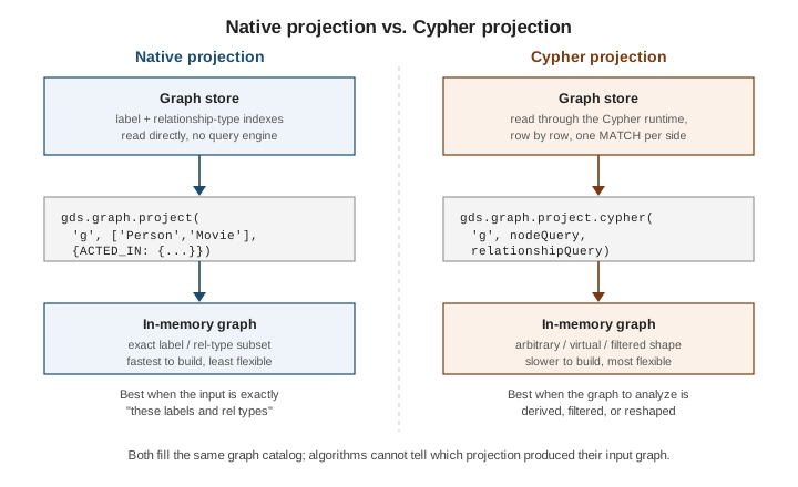
Native projection — declared as label/relationship-type filters plus a property list, as in the example above. It reads directly from the store’s internal structures, so it projects fastest and scales to the largest graphs, but it can only select by label and relationship type, and any derived or computed values are not available.
-
Cypher projection — declared as a
MATCH-based query that returns arbitrary node and relationship rows, letting the projected graph be a filtered subset, a reshaped set of "virtual" relationships (e.g. a multi-hop path collapsed into one edge), or the result of arbitrary property computation. It is far more flexible but slower to build, since every row is evaluated through the Cypher runtime rather than read straight off disk.
// Cypher projection: collapse Person -[:ACTED_IN]-> Movie <-[:ACTED_IN]- Person
// into a single virtual CO_ACTED_WITH relationship between co-stars
CALL gds.graph.project.cypher(
  'co-actors',
  'MATCH (p:Person) RETURN id(p) AS id',
  'MATCH (p1:Person)-[:ACTED_IN]->(:Movie)<-[:ACTED_IN]-(p2:Person)
   WHERE id(p1) < id(p2)
   RETURN id(p1) AS source, id(p2) AS target, count(*) AS weight'
)
YIELD graphName, nodeCount, relationshipCount
RETURN graphName, nodeCount, relationshipCount
Reach for a native projection whenever the algorithm’s input graph is exactly "these labels and
relationship types" — it is the default and should stay the default. Reach for a Cypher projection only
when the graph to analyze does not exist as a direct label/relationship pattern — a derived edge, a
filtered subset expressed with WHERE, or a graph built from a query that spans several relationship
hops
(GDS Introduction).
Execution modes: stream, mutate, write, stats
Every GDS algorithm ships as a family of procedures that share one algorithm implementation but differ in what happens to the result:
| Mode | Behavior |
|---|---|
|
Returns each result row directly to the caller. Nothing is persisted anywhere — use it to inspect results or feed them into further Cypher in the same query. |
|
Writes the result back onto the in-memory projected graph as a new node or relationship property, so a later algorithm in the same catalog entry can consume it without re-projecting. |
|
Persists the result back to the stored graph in the database as a node or relationship property, visible to ordinary Cypher queries once it completes. |
|
Returns only summary statistics about what the algorithm would produce (counts, timings, distribution percentiles) without returning or persisting any per-node result. |
// Same algorithm, four modes, against the "people-movies" graph
CALL gds.pageRank.stream('people-movies')
YIELD nodeId, score
RETURN gds.util.asNode(nodeId).name AS name, score
ORDER BY score DESC LIMIT 5;

CALL gds.pageRank.mutate('people-movies', { mutateProperty: 'pageRank' })
YIELD nodePropertiesWritten;

CALL gds.pageRank.write('people-movies', { writeProperty: 'pageRank' })
YIELD nodePropertiesWritten;

CALL gds.pageRank.stats('people-movies')
YIELD centralityDistribution
RETURN centralityDistribution;
A common pipeline chains mutate calls across several algorithms on the same in-memory graph — each
algorithm’s output becomes the next one’s input property — and only calls write once, at the end, to
persist the final derived properties back to the database
(GDS Algorithms).
Dropping graphs and estimating memory
A projected graph occupies heap memory for as long as it stays in the catalog. Drop it explicitly once the analysis is done rather than waiting for the database to restart:
CALL gds.graph.drop('people-movies') YIELD graphName;Because a projection is built entirely in memory, projecting a graph that does not fit crashes the
operation partway through. gds.graph.project.estimate runs the same projection logic against the
catalog’s cost model without allocating anything, returning the memory it would require so the projection
can be sized — or the instance upgraded — before committing to it:
CALL gds.graph.project.estimate(
  ['Person', 'Movie'],
  { ACTED_IN: { orientation: 'NATURAL' } }
)
YIELD requiredMemory, nodeCount, relationshipCount
RETURN requiredMemory, nodeCount, relationshipCount
Most individual algorithm procedures accept the same graph configuration with an .estimate suffix as
well (e.g. gds.pageRank.write.estimate), so both the projection and the algorithm run’s memory can be
checked ahead of time
(GDS Getting Started).
Algorithm categories
GDS ships four broad families of algorithms, all built on the catalog and execution modes above. Each has its own dedicated page in this section.
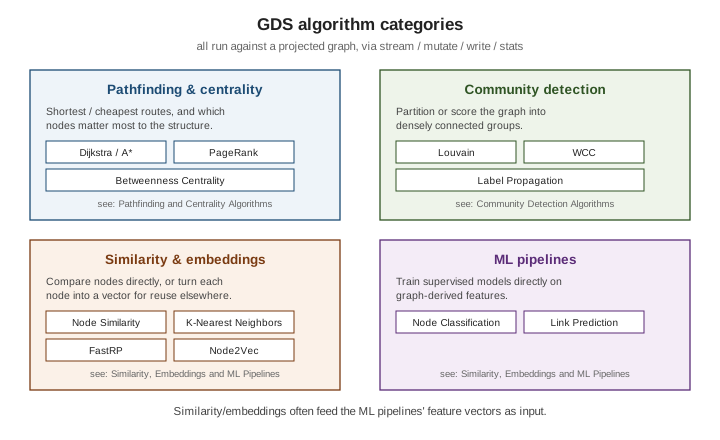
Pathfinding and centrality algorithms answer "what is the shortest/cheapest route between these nodes" and "which nodes matter most to the graph’s structure" — Dijkstra, A*, and centrality measures such as PageRank and Betweenness Centrality. See Pathfinding and Centrality Algorithms.
Community detection algorithms partition or score the graph into densely connected groups — Louvain, Weakly Connected Components, and Label Propagation are the most common entry points. See Community Detection Algorithms.
Similarity algorithms compare nodes to each other directly (Node Similarity, K-Nearest Neighbors), while node embeddings (FastRP, Node2Vec) turn each node into a numeric vector for downstream similarity search or machine learning, and the ML pipelines feature trains supervised models — node classification, link prediction — directly on top of those graph-derived features. See Similarity, Embeddings and ML Pipelines.
Related pages
-
GDS Documentation — the full library reference this page summarizes.
-
GDS Introduction — the catalog and projection concepts in more depth.
-
GDS Getting Started — installing the plugin and running a first algorithm end to end.
-
GDS Algorithms — the full algorithm catalog behind the category pages linked above.
-
Cypher Fundamentals — the query language used to build Cypher projections.