Vector Indexing & HNSW

This section documents the current Qdrant 1.x line (latest 1.19.1), written and verified against the official Qdrant documentation. No specific patch version is pinned. Some capabilities (Qdrant Cloud-only features and the full breadth of client-library APIs beyond Python and Java) are linked, not documented in depth.

This content was generated with the assistance of AI and should be verified against the official documentation before being relied on in production.

This section’s bibliography lists the reference material consulted while preparing these pages.

Every Qdrant collection — or, with multiple named vectors, every vector within it — keeps its own HNSW graph: a layered proximity structure that turns nearest-neighbor search from a full scan into a greedy walk from a sparse top layer down to a bottom layer holding every point. This page covers the parameters that shape that graph, the knob that trades recall for latency at query time without touching the index, the escape hatch to exact brute-force search, and the quantization schemes Qdrant offers to shrink memory and speed up scoring.

The HNSW index

Qdrant builds one HNSW graph per collection by default, or one per named vector when a collection defines several (each named vector can even set its own hnsw_config, so a small metadata vector and a large embedding vector in the same collection are not forced to share graph parameters). Below a configurable vector data size (full_scan_threshold_kb, in KB of raw vector data) Qdrant skips the graph and scans directly, since building and walking an index costs more than it saves on a handful of vectors.

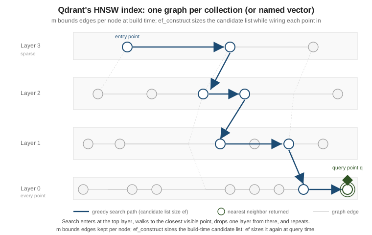
The full set of index parameters — including the payload indexes covered on the next page — is described in Indexing.

`hnsw_config`: `m` and `ef_construct`

Two parameters control the graph Qdrant builds:

Parameter Meaning

Parameter	Meaning
`m`	Maximum edges kept per node (per layer). Higher `m` raises recall and makes the graph more robust to badly-placed entry points, at the cost of more memory per point and a slower build; very low `m` (below around 4) degrades recall sharply. Default is `16`.
`ef_construct`	Size of the candidate list explored while wiring each new point into the graph. A larger `ef_construct` finds better neighbors for that point — improving recall — but makes indexing slower; it does not change search latency once the graph is built, only how good the graph is. Default is `100`.

m

Maximum edges kept per node (per layer). Higher m raises recall and makes the graph more robust to badly-placed entry points, at the cost of more memory per point and a slower build; very low m (below around 4) degrades recall sharply. Default is 16.

ef_construct

Size of the candidate list explored while wiring each new point into the graph. A larger ef_construct finds better neighbors for that point — improving recall — but makes indexing slower; it does not change search latency once the graph is built, only how good the graph is. Default is 100.

Both are set in hnsw_config, either globally for the collection or per named vector, at collection creation time (and can be changed later, which triggers a rebuild of the affected graph):

// PUT /collections/documents
{
  "vectors": {
    "size": 768,
    "distance": "Cosine"
  },
  "hnsw_config": {
    "m": 16,
    "ef_construct": 200,
    "full_scan_threshold_kb": 20000
  }
}

A collection with multiple named vectors can override hnsw_config per vector, e.g. a higher m for the vector that carries most of the search traffic:

// PUT /collections/catalog
{
  "vectors": {
    "image": { "size": 512, "distance": "Cosine" },
    "text": {
      "size": 1536,
      "distance": "Cosine",
      "hnsw_config": { "m": 32, "ef_construct": 256 }
    }
  }
}

Raising both parameters is the standard way to buy recall with more build time and memory; the reference trade-off table lives on the same Indexing page.

Search-time `ef`

Search quality against an already-built graph is governed by a third parameter, ef (named hnsw_ef in the search-request parameters), which is completely independent of the two build-time settings above: it is the size of the candidate list the greedy walk keeps while answering one query, not while building the index. A larger ef visits more candidates per layer, raising recall at the cost of latency; a smaller ef answers faster but may miss true neighbors. Because it lives in the search request rather than the collection’s index configuration, ef can be tuned per query — or even per client — with no rebuild:

from qdrant_client import QdrantClient
from qdrant_client.http import models

client = QdrantClient(url="http://localhost:6333")

hits = client.query_points(
    collection_name="documents",
    query=query_vector,
    limit=10,
    search_params=models.SearchParams(
        hnsw_ef=256,   # candidate list size for this query only
        exact=False,
    ),
)

Exact vs. approximate search

HNSW search is approximate: the greedy walk is not guaranteed to find the true nearest neighbors, only a close set with high probability. For small collections, or to compute ground-truth results to measure how much recall a given ef/m/ef_construct combination is actually losing, Qdrant can bypass the graph entirely and score every point by brute force via the same exact flag shown above:

ground_truth = client.query_points(
    collection_name="documents",
    query=query_vector,
    limit=10,
    search_params=models.SearchParams(exact=True),  # forces brute-force search
)

Because exact is a per-request flag, a single collection can serve fast approximate search for normal traffic and exact search on demand for evaluation, without maintaining a second index.

Quantization

Quantization trades some vector precision for a smaller memory footprint and faster distance computations, and is configured on the collection (or per named vector) alongside hnsw_config. Qdrant offers three schemes, described in full in Quantization:

Scheme	What it trades away	Reach for it when
Scalar (int8)	Each float32 component is quantized to a single byte, roughly a 4x memory reduction with a small, usually negligible recall loss.	The default choice for shrinking memory on float32 collections without much tuning.
Product	Vectors are split into sub-vectors, each replaced by the id of its nearest entry in a learned codebook, giving the largest compression ratios of the three.	Memory is the dominant constraint and a larger recall/CPU cost (codebook lookups are slower than scalar math) is acceptable.
Binary	Each component is reduced to a single bit, giving up to a 32x memory reduction and the fastest possible distance computation (a Hamming distance).	High-dimensional embeddings from modern large models (1024+ dimensions), where the extra dimensionality means the recall hit from binarizing is typically small — often the best memory/speed win of the three for that case.

Scheme

What it trades away

Reach for it when

Scalar (int8)

Each float32 component is quantized to a single byte, roughly a 4x memory reduction with a small, usually negligible recall loss.

The default choice for shrinking memory on float32 collections without much tuning.

Product

Vectors are split into sub-vectors, each replaced by the id of its nearest entry in a learned codebook, giving the largest compression ratios of the three.

Memory is the dominant constraint and a larger recall/CPU cost (codebook lookups are slower than scalar math) is acceptable.

Binary

Each component is reduced to a single bit, giving up to a 32x memory reduction and the fastest possible distance computation (a Hamming distance).

High-dimensional embeddings from modern large models (1024+ dimensions), where the extra dimensionality means the recall hit from binarizing is typically small — often the best memory/speed win of the three for that case.

All three are configured through quantization_config at collection-creation (or update) time; Qdrant still keeps the original vectors on disk by default and uses the quantized form only to narrow the candidate set, optionally rescoring with the full vectors before returning results:

client.create_collection(
    collection_name="embeddings",
    vectors_config=models.VectorParams(size=1536, distance=models.Distance.COSINE),
    hnsw_config=models.HnswConfigDiff(m=16, ef_construct=200),
    quantization_config=models.BinaryQuantization(
        binary=models.BinaryQuantizationConfig(always_ram=True),
    ),
)

# scalar quantization is the lighter-touch alternative:
client.update_collection(
    collection_name="documents",
    quantization_config=models.ScalarQuantization(
        scalar=models.ScalarQuantizationConfig(
            type=models.ScalarType.INT8,
            quantile=0.99,
            always_ram=True,
        ),
    ),
)

Where to go next

Collections & Points — how the collections and named vectors indexed here are created and populated.
Filtering & Payload Indexing — payload indexes and how filters interact with the HNSW graph walk.
kNN / HNSW vector search — Lucene’s own HNSW codec, Lucene99HnswVectorsFormat, tunes the same trade-off through maxConn/beamWidth instead of Qdrant’s m/ef_construct.
Vector & semantic search — Elasticsearch exposes the same graph through dense_vector and index_options, where Qdrant uses a dedicated hnsw_config block.
ANN Indexes: Flat, IVF, HNSW and Beyond and Quantization & Compression — the vendor-neutral theory behind HNSW, IVF and vector quantization, of which this page is Qdrant’s implementation.