ANN Indexes: Flat, IVF, HNSW and Beyond

This content was generated with the assistance of AI and should be verified against the official documentation of each tool and framework before being relied on in production.

This section’s bibliography lists the reference material consulted while preparing these pages.

This page’s runnable examples target Python 3.12 and FAISS 1.15.1. They build ANN indexes over the DocsAssistant scenario’s 768-dimension embeddings (Ollama nomic-embed-text), and compare an IndexHNSWFlat against the IndexFlatIP ground truth that later pages also use for recall measurement.

The approximate nearest neighbor problem

Exact nearest-neighbor search over vectors — scoring every stored vector against the query and keeping the top k — is a linear scan: correct, but its cost grows with the number of vectors, n. Once a collection holds millions of embeddings, scanning all of them for every query is too slow for interactive search. Approximate nearest neighbor (ANN) search accepts a small, controllable chance of returning a vector that is not the true nearest neighbor in exchange for sub-linear query time.

Formally, an index solves the -approximate nearest neighbor problem when, for a query point and a true nearest neighbor at distance , it returns a point within distance :

is exact search; larger allows the index to skip more of the search space and return slightly worse matches faster. In practice no production index measures directly — it is a theoretical framing — but every tunable parameter on this page (nprobe, efSearch, and so on) moves the same dial: how much of the true neighborhood the search is willing to miss in exchange for speed.

The trade-off axes

Every ANN index is a point in a four-way trade-off, and no configuration wins on all four at once:

Axis What it measures

Axis	What it measures
Recall@k	The fraction of the true top-`k` neighbors (from an exact search) that the approximate search actually returns. The standard way to quantify "how approximate."
Query latency	Time to answer one query. Usually the axis being optimized for, since it is what users and agents feel.
Memory	Bytes held per vector: the raw vector plus whatever index structure (graph edges, inverted lists, hash tables) the algorithm keeps alongside it.
Build time	Time to construct the index from a batch of vectors (or to insert one more vector into an existing index). Matters for both initial ingestion and index maintenance.

Recall@k

The fraction of the true top-k neighbors (from an exact search) that the approximate search actually returns. The standard way to quantify "how approximate."

Query latency

Time to answer one query. Usually the axis being optimized for, since it is what users and agents feel.

Memory

Bytes held per vector: the raw vector plus whatever index structure (graph edges, inverted lists, hash tables) the algorithm keeps alongside it.

Build time

Time to construct the index from a batch of vectors (or to insert one more vector into an existing index). Matters for both initial ingestion and index maintenance.

Raising recall almost always costs latency, memory, or build time — usually more than one of the three. Tuning an ANN index is choosing where on this frontier a given workload needs to sit, not finding a setting that is simply "better."

The curse of dimensionality

ANN indexes exploit spatial structure — neighborhoods, clusters, locality — and that structure grows weaker as dimensionality rises. In very high dimensions, distances between random points concentrate: the ratio between the nearest and farthest neighbor’s distance to a query shrinks toward 1, so "nearest" stops being a sharply distinguishing property. This curse of dimensionality is why brute-force exact search degrades gracefully with dimension while some ANN structures (LSH in particular) need exponentially more hash tables to keep recall stable as dimensionality grows, and why modern embedding models keep dimensions in the hundreds to low thousands rather than much higher — Embeddings and Quantization & Compression cover the dimension/quality/memory trade-off directly.

Flat: exact search as the baseline

A flat (or brute-force) index stores every vector as-is and, for each query, computes the distance to every stored vector. It is always exact (recall@k = 1.0 by construction) and needs no training or tuning, which makes it the correct choice for small collections and the mandatory ground truth against which every approximate index’s recall is measured:

import faiss
import numpy as np

d = 768
xb = np.random.default_rng(0).random((10_000, d), dtype=np.float32)
faiss.normalize_L2(xb)  # cosine similarity via normalized inner product

index_flat = faiss.IndexFlatIP(d)
index_flat.add(xb)

xq = xb[:5]  # pretend these are query vectors
distances, ids = index_flat.search(xq, k=10)

See Faiss indexes for IndexFlatIP and its L2 sibling IndexFlatL2.

IVF: inverted file indexes

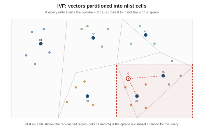
An IVF (inverted file) index partitions the vector space into nlist clusters using k-means, then, at search time, only scores the vectors inside the nprobe clusters whose centroids are closest to the query — instead of every vector in the collection. It needs a training step (running k-means on a representative sample) before vectors can be added, and its recall depends heavily on how evenly the data falls into clusters:

Parameter Meaning

Parameter	Meaning
`nlist`	Number of k-means clusters (inverted lists) the space is partitioned into. More clusters means each one is smaller and cheaper to scan fully, but more clusters must be checked to keep recall up.
`nprobe`	Number of nearest clusters actually scanned per query. `nprobe = nlist` degrades to an exact scan; `nprobe = 1` is fastest and least accurate. This is IVF’s main recall/latency knob, analogous to HNSW’s `efSearch` below.

nlist

Number of k-means clusters (inverted lists) the space is partitioned into. More clusters means each one is smaller and cheaper to scan fully, but more clusters must be checked to keep recall up.

nprobe

Number of nearest clusters actually scanned per query. nprobe = nlist degrades to an exact scan; nprobe = 1 is fastest and least accurate. This is IVF’s main recall/latency knob, analogous to HNSW’s efSearch below.

nlist = 64
quantizer = faiss.IndexFlatIP(d)
index_ivf = faiss.IndexIVFFlat(quantizer, d, nlist, faiss.METRIC_INNER_PRODUCT)

index_ivf.train(xb)      # k-means over nlist clusters -- required before add()
index_ivf.add(xb)

index_ivf.nprobe = 8      # scan 8 of the 64 clusters per query
distances, ids = index_ivf.search(xq, k=10)

Cluster skew is IVF’s main failure mode: if the data is not uniformly distributed, some clusters end up much larger than others (a common outcome with real embeddings, which cluster around topics), so a fixed nprobe scans a wildly uneven number of vectors depending on which clusters a query lands near, and outlier queries near sparse clusters can miss neighbors that a differently-clustered dataset would have found. Re-training on a larger, more representative sample, or raising nlist to shrink each cluster, are the usual mitigations. See Cell-probe methods (IndexIVF* indexes).

In pgvector the same structure is an ivfflat index, with lists playing the role of nlist and ivfflat.probes the role of nprobe. The DocsAssistant schema uses HNSW (below), so this is the IVF alternative on the same table:

CREATE INDEX chunk_embeddings_ivfflat ON chunk_embeddings
    USING ivfflat (embedding vector_cosine_ops) WITH (lists = 64);  -- build after loading data

SET ivfflat.probes = 8;  -- per session; the default is 1
SELECT chunk_id FROM chunk_embeddings ORDER BY embedding <=> $1 LIMIT 10;

See pgvector README — IVFFlat.

LSH

Locality-sensitive hashing (LSH) takes a different approach: it hashes vectors with functions chosen so that nearby vectors collide into the same bucket with high probability, then only compares candidates sharing a bucket with the query. It needs no training, but as dimensionality grows LSH needs more hash tables to keep recall stable, which is one concrete face of the curse of dimensionality above.

FAISS ships a random-projection variant as IndexLSH: each vector is projected onto nbits random hyperplanes and stored as a binary code, one bit per hyperplane, and a query is compared with every stored code by Hamming distance. The number of matching bits approximates the angle between the vectors, so it pairs naturally with normalized, cosine-style embeddings; more bits give a closer approximation at the cost of more memory:

nbits = 2 * d  # 1536 bits = 192 bytes per vector, versus 3072 bytes as float32
index_lsh = faiss.IndexLSH(d, nbits)
index_lsh.add(xb)  # no training needed
distances, ids = index_lsh.search(xq, k=10)  # distances are Hamming distances between codes

See Faiss indexes for IndexLSH. In practice, IVF and HNSW have largely displaced LSH for dense embedding search because they scale better with dimension, and LSH is now mostly seen in older systems or as a building block for specific hashing schemes (and for binary codes, see Quantization & Compression) rather than as the default ANN structure.

HNSW: hierarchical navigable small world graphs

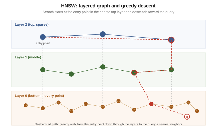
HNSW builds a multi-layer graph where each vector is a node connected to its approximate nearest neighbors. The top layer is sparse and covers long distances across the space; each lower layer is progressively denser, until the bottom layer contains every point. A search starts at an entry point in the top layer and greedily walks toward the query, descending a layer whenever the current layer’s local neighborhood stops improving — so most of the distance is covered cheaply in the sparse layers, and only the final, precise steps happen in the dense bottom layer.

Vector Indexing & HNSW documents this same structure as Qdrant configures it (hnsw_config’s `m / ef_construct, and per-query ef) — this page uses FAISS’s names for the same three parameters:

Parameter Meaning

Parameter	Meaning
`M`	Maximum edges kept per node per layer. Higher `M` gives a more richly connected, higher-recall graph at the cost of more memory per vector and slower inserts. A bare `HNSW` in a FAISS `index_factory` string uses `32`; Qdrant’s collection default and pgvector’s default are `16` — all are reasonable starting points, and the DocsAssistant scenario uses `M = 16` in both FAISS (`IndexHNSWFlat(768, 16)`) and pgvector (`m = 16`).
`efConstruction`	Candidate-list size explored while wiring a new node into the graph at build time. Larger values build a better graph (more likely to find each node’s true near neighbors) at the cost of slower inserts; it has no effect on search latency once the graph exists.
`efSearch`	Candidate-list size kept while walking the graph for one query. This is HNSW’s main recall/latency knob, tuned per query with no rebuild — the same role `nprobe` plays for IVF.

M

Maximum edges kept per node per layer. Higher M gives a more richly connected, higher-recall graph at the cost of more memory per vector and slower inserts. A bare HNSW in a FAISS index_factory string uses 32; Qdrant’s collection default and pgvector’s default are 16 — all are reasonable starting points, and the DocsAssistant scenario uses M = 16 in both FAISS (IndexHNSWFlat(768, 16)) and pgvector (m = 16).

efConstruction

Candidate-list size explored while wiring a new node into the graph at build time. Larger values build a better graph (more likely to find each node’s true near neighbors) at the cost of slower inserts; it has no effect on search latency once the graph exists.

efSearch

Candidate-list size kept while walking the graph for one query. This is HNSW’s main recall/latency knob, tuned per query with no rebuild — the same role nprobe plays for IVF.

M = 16
index_hnsw = faiss.IndexHNSWFlat(d, M, faiss.METRIC_INNER_PRODUCT)
index_hnsw.hnsw.efConstruction = 64
index_hnsw.add(xb)              # no training step needed, unlike IVF

index_hnsw.hnsw.efSearch = 64
distances, ids = index_hnsw.search(xq, k=10)

See HNSW indexes on the FAISS wiki, and the original algorithm in Malkov & Yashunin, "Efficient and robust approximate nearest neighbor search using Hierarchical Navigable Small World graphs".

In pgvector the same three parameters are m and ef_construction on the index and the hnsw.ef_search setting at query time. This is the DocsAssistant scenario’s own index on chunk_embeddings:

CREATE INDEX chunk_embeddings_hnsw ON chunk_embeddings
    USING hnsw (embedding vector_cosine_ops) WITH (m = 16, ef_construction = 64);

SET hnsw.ef_search = 64;  -- per session (or SET LOCAL per transaction); the default is 40
SELECT chunk_id FROM chunk_embeddings ORDER BY embedding <=> $1 LIMIT 10;

See pgvector README — HNSW and PostgreSQL & pgvector for the full schema.

Memory per vector

HNSW’s memory cost is the raw vector plus its graph edges. For a d-dimension float32 vector with M edges per node (FAISS keeps roughly 2*M edges per node across levels, each stored as a 4-byte identifier), the per-vector footprint is approximately:

For the DocsAssistant scenario’s with , that is bytes per vector — roughly 4% overhead above the 3072 raw bytes. This formula reappears on Comparing Vector Databases for a full capacity worked example, and its first term ( ) is also where the quantization schemes on Quantization & Compression cut memory, since they shrink each component’s byte size without changing M.

Insert, delete and complexity

HNSW supports incremental inserts naturally: a new node is wired into the existing layers using the same greedy search used for queries, without touching the rest of the graph. Deletion is the weaker operation: most implementations (including FAISS’s IndexHNSWFlat) do not support removing a node’s edges cleanly, so a "deleted" vector is instead marked as a tombstone and filtered out of results, or the graph is periodically rebuilt to reclaim it. This asymmetry is one reason engines built around HNSW (Qdrant, the pgvector extension) favor soft-delete-and-compact patterns over in-place edge removal.

Search complexity is commonly quoted as , and the greedy multi-layer walk is designed to behave that way in the regime the original paper targets: uniformly distributed, moderate-dimension data with a large enough graph that the layer structure actually thins out neighborhoods. In practice " " is a heuristic, not a guarantee — highly clustered real-world embeddings, very high dimensionality (where the curse of dimensionality above weakens the locality the graph relies on), or a poorly tuned M/efConstruction can push actual behavior toward something closer to linear in the worst case. Treat the log-like scaling as an empirical property to verify with a recall/latency benchmark on real data (FAISS and Comparing Vector Databases both build one), not as an algorithmic guarantee.

Beyond in-memory HNSW: DiskANN, Vamana and disk-based indexes

HNSW keeps its whole graph in memory, which becomes expensive at the billion-vector scale (the memory formula above, multiplied out, adds up fast). DiskANN and its underlying Vamana graph algorithm take a different design point: build a single-layer, carefully pruned graph sized to live mostly on SSD, and use the disk’s high random-read throughput — rather than RAM — to hold most vectors, keeping only a small in-memory routing structure (and often a compressed copy of each vector, for cheap approximate scoring before a final disk read confirms the candidate). This buys much larger indexes per dollar of RAM at the cost of higher per-query I/O latency than a fully in-memory HNSW graph.

The Vamana graph is also useful in memory: its single, flat graph plus compressed vectors can need less RAM than an HNSW graph over full-precision vectors. Several engines now offer an alternative to in-memory HNSW along one of these two lines — a Vamana graph, or an index that lives mostly on disk:

Engine Option Where the index lives

Engine	Option	Where the index lives
Redis Query Engine	`SVS-VAMANA` (Intel’s Scalable Vector Search), added in Redis 8.2 — see Vector Search: Query Engine & Vector Sets	In memory. Its `LVQ`/`LeanVec` compression shrinks the RAM each vector needs; it does not move the graph to SSD, so it is not a fit for data larger than RAM.
Milvus	`DiskANN` index type — Milvus DiskANN index	On local SSD, with compressed vectors in memory for routing; built for collections too large to fit in memory.
Couchbase	The Hyperscale vector index — Hyperscale Vector Index	Disk-based: it keeps its data in an optimized on-disk format (partitioned IVF-style around centroids), so it needs far less memory than an in-memory index.
PostgreSQL	`pg_diskann`, an extension implementing the Vamana graph for Postgres, offered as an alternative to pgvector’s in-memory HNSW on some managed services (see PostgreSQL & pgvector) — `pg_diskann` on GitHub	In PostgreSQL’s own disk pages, read through the buffer cache like any other index.

Redis Query Engine

SVS-VAMANA (Intel’s Scalable Vector Search), added in Redis 8.2 — see Vector Search: Query Engine & Vector Sets

In memory. Its LVQ/LeanVec compression shrinks the RAM each vector needs; it does not move the graph to SSD, so it is not a fit for data larger than RAM.

Milvus

DiskANN index type — Milvus DiskANN index

On local SSD, with compressed vectors in memory for routing; built for collections too large to fit in memory.

Couchbase

The Hyperscale vector index — Hyperscale Vector Index

Disk-based: it keeps its data in an optimized on-disk format (partitioned IVF-style around centroids), so it needs far less memory than an in-memory index.

PostgreSQL

pg_diskann, an extension implementing the Vamana graph for Postgres, offered as an alternative to pgvector’s in-memory HNSW on some managed services (see PostgreSQL & pgvector) — pg_diskann on GitHub

In PostgreSQL’s own disk pages, read through the buffer cache like any other index.

The original algorithm and its disk-resident design are described in Subramanya et al., "DiskANN: Fast Accurate Billion-point Nearest Neighbor Search on a Single Node".

Choosing an index

flowchart TD A[How many vectors?] -->|"< ~100K"| B[Flat: exact, no tuning needed] A -->|"100K - low millions"| C{RAM budget tight?} A -->|"tens of millions or more"| D{Fits in RAM with M edges?} C -->|No| E[HNSW: best recall/latency trade-off] C -->|Yes, very tight| F[IVF: coarser but smaller footprint] D -->|Yes| E D -->|No| G[DiskANN / Vamana: disk-resident graph] E --> H{Need to shrink memory further?} H -->|Yes| I[Add quantization: scalar, PQ or binary] H -->|No| J[Done]

As a rule of thumb: reach for Flat while a collection is small enough that exact search is fast and tuning would be wasted effort; reach for IVF when memory is the binding constraint and a coarser recall profile is acceptable; reach for HNSW as the default for most production, RAM-resident collections needing low-latency approximate search; and reach for a DiskANN/Vamana variant once the collection is too large to keep an HNSW-style graph in RAM at all. Quantization & Compression covers combining any of these with scalar, product or binary quantization to push the memory budget further, and Comparing Vector Databases extends this decision with per-engine cost and operational trade-offs.

Parameter equivalence across engines

Every engine implements the same handful of IVF/HNSW knobs under its own names. Recognizing the correspondence is what makes tuning advice from one engine’s docs transferable to another:

Concept Engine parameter

Concept	Engine parameter
HNSW build-time edges (`M`)	pgvector `m` (PostgreSQL & pgvector); Qdrant `hnsw_config.m` (Vector Indexing & HNSW); Redis `M` (Vector Search: Query Engine & Vector Sets); Elasticsearch `index_options.m` (Vector & semantic search); Lucene `maxConn` (kNN / HNSW vector search); Milvus `M` in its `HNSW` index params; FAISS `M`.
HNSW build-time candidate list	pgvector `ef_construction`; Qdrant `hnsw_config.ef_construct`; Redis `EF_CONSTRUCTION`; Elasticsearch `index_options.ef_construction`; Lucene `beamWidth`; Milvus `efConstruction`; FAISS `efConstruction`.
HNSW search-time candidate list	pgvector `SET hnsw.ef_search`; Qdrant per-query `hnsw_ef`; Redis `EF_RUNTIME`; Elasticsearch `num_candidates`; Lucene per-query `k` and visited-node budget; Milvus `ef` search param; FAISS `efSearch`.
IVF cluster count	pgvector ivfflat’s `lists; FAISS `nlist`; Milvus `nlist` in its `IVF_FLAT`/ `IVF_PQ` params.
IVF probe count	pgvector `SET ivfflat.probes`; FAISS `nprobe`; Milvus `nprobe` search param.

HNSW build-time edges (M)

pgvector m (PostgreSQL & pgvector); Qdrant hnsw_config.m (Vector Indexing & HNSW); Redis M (Vector Search: Query Engine & Vector Sets); Elasticsearch index_options.m (Vector & semantic search); Lucene maxConn (kNN / HNSW vector search); Milvus M in its HNSW index params; FAISS M.

HNSW build-time candidate list

pgvector ef_construction; Qdrant hnsw_config.ef_construct; Redis EF_CONSTRUCTION; Elasticsearch index_options.ef_construction; Lucene beamWidth; Milvus efConstruction; FAISS efConstruction.

HNSW search-time candidate list

pgvector SET hnsw.ef_search; Qdrant per-query hnsw_ef; Redis EF_RUNTIME; Elasticsearch num_candidates; Lucene per-query k and visited-node budget; Milvus ef search param; FAISS efSearch.

IVF cluster count

pgvector ivfflat’s `lists; FAISS nlist; Milvus nlist in its IVF_FLAT/ IVF_PQ params.

IVF probe count

pgvector SET ivfflat.probes; FAISS nprobe; Milvus nprobe search param.

The following FAISS snippet measures recall@10 as a function of efSearch against the IndexFlatIP ground truth built earlier, which is the same methodology FAISS and Comparing Vector Databases use for their own benchmarks:

import faiss
import numpy as np

rng = np.random.default_rng(42)
d, n, n_queries, k = 768, 50_000, 200, 10

xb = rng.random((n, d), dtype=np.float32)
xq = rng.random((n_queries, d), dtype=np.float32)
faiss.normalize_L2(xb)
faiss.normalize_L2(xq)

# ground truth
index_flat = faiss.IndexFlatIP(d)
index_flat.add(xb)
_, ground_truth_ids = index_flat.search(xq, k)

# approximate index under test
index_hnsw = faiss.IndexHNSWFlat(d, 16, faiss.METRIC_INNER_PRODUCT)
index_hnsw.hnsw.efConstruction = 64
index_hnsw.add(xb)


def recall_at_k(approx_ids: np.ndarray, exact_ids: np.ndarray) -> float:
    hits = sum(
        len(set(approx_ids[i]) & set(exact_ids[i]))
        for i in range(len(exact_ids))
    )
    return hits / (len(exact_ids) * exact_ids.shape[1])


for ef_search in (16, 32, 64, 128, 256):
    index_hnsw.hnsw.efSearch = ef_search
    _, approx_ids = index_hnsw.search(xq, k)
    print(f"efSearch={ef_search:4d}  recall@{k} = {recall_at_k(approx_ids, ground_truth_ids):.3f}")

Running this prints recall@10 rising toward 1.0 as efSearch grows — the exact numbers depend on the random data and are not reported here as facts, per this section’s "no invented numbers" rule. See HNSW indexes and Guidelines to choose an index on the FAISS wiki.

IVF cells, visually

A 2-D scatter of points partitioned into Voronoi-like IVF cells around k-means centroids, with a query point and the nprobe = 2 nearest cells highlighted for scanning

In LangChain and Spring AI

LangChain

langchain-postgres’s `PGVector does not create an ANN index or expose HNSW/IVF parameters: it creates its own tables (langchain_pg_collection and langchain_pg_embedding) and searches them with an exact scan until you add an index yourself. Passing embedding_length gives the embedding column a fixed dimension, which pgvector requires before it can index it; the index is then the same SQL as on the hand-written schema above, pointed at the framework’s table:

from langchain_ollama import OllamaEmbeddings
from langchain_postgres import PGVector

vector_store = PGVector(
    embeddings=OllamaEmbeddings(model="nomic-embed-text"),
    embedding_length=768,  # vector(768) instead of an unsized vector column
    collection_name="docsassistant",
    connection="postgresql+psycopg://docs:docs@localhost:5432/docsassistant",
    use_jsonb=True,
)

-- run once against the framework-managed table (default distance strategy: cosine)
CREATE INDEX langchain_pg_embedding_hnsw ON langchain_pg_embedding
    USING hnsw (embedding vector_cosine_ops) WITH (m = 16, ef_construction = 64);

See the official LangChain PGVector page and LangChain vector stores.

Spring AI

PgVectorStore exposes the index type as configuration — index-type is NONE (exact scan, no index), IVFFLAT or HNSW (the default) — and creates that index when initialize-schema is true. It has no properties for m, ef_construction or lists: to use non-default HNSW parameters, set initialize-schema: false and create the table and index yourself with the SQL shown above, and set hnsw.ef_search in SQL too (per session or per database):

spring:
  ai:
    vectorstore:
      pgvector:
        table-name: docs_vector_store
        index-type: HNSW
        distance-type: COSINE_DISTANCE
        dimensions: 768
        initialize-schema: true

See the official Spring AI PGvector page and Spring AI vector store API.

Vector Indexing & HNSW — HNSW as Qdrant configures and tunes it per collection.
kNN / HNSW vector search — Lucene’s HNSW codec (maxConn / beamWidth) and its quantized vector formats.
Vector Search: Query Engine & Vector Sets — FLAT, HNSW and SVS-VAMANA on the Redis Query Engine.
Vector & semantic search — dense_vector and index_options.
Quantization & Compression — shrinking the memory formula above with scalar, product and binary quantization.
FAISS — FAISS as a library, and a fuller Flat/IVF/HNSW benchmark.
PostgreSQL & pgvector — pgvector’s own HNSW and IVFFlat configuration.
Comparing Vector Databases — the capacity/cost worked example built on this page’s memory formula.