Hybrid Search & Re-ranking
|
This content was generated with the assistance of AI and should be verified against the official documentation of each tool and framework before being relied on in production. This section’s bibliography lists the reference material consulted while preparing these pages. |
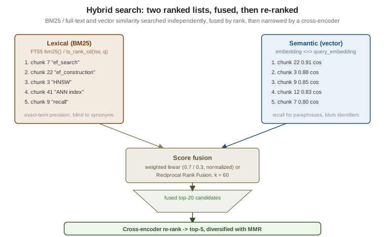
Examples on this page target Python 3.12, sentence-transformers 6.1, PostgreSQL 17 with pgvector 0.8.6, SQLite with the FTS5 extension, langchain / langchain-classic 1.4, and Spring Boot 4.1 with Spring AI 2.0.1. Pure vector similarity and pure keyword search each miss things the other catches; hybrid search runs both and combines the results, and re-ranking spends a second, more expensive pass narrowing that combined list down to the handful of chunks that actually go into the prompt.
Why vectors blur exact terms
An embedding model represents meaning, not characters. ef_search and efSearch land close together in
vector space because they mean the same thing, but so do ef_search and ef_construction, because both
sentences are "about HNSW tuning parameters" — the embedding has no notion that only one of them is the
exact identifier the user typed. A query such as "what does ef_search control" over the DocsAssistant
corpus can retrieve a chunk that discusses ef_construction at a higher cosine similarity than the chunk
that actually defines ef_search, simply because the two parameters co-occur in the same paragraphs.
Anything an embedding model was not trained to distinguish precisely — code identifiers, product SKUs, error
codes, version numbers, acronyms — is exactly where a classic keyword ranking function still wins, which is
why hybrid search runs both and lets each cover the other’s blind spot.
BM25 over SQLite FTS5
BM25 scores a document higher the more it repeats a query term, but with saturation (the fifth occurrence
of a term adds much less than the second) and length normalization (a hit in a short chunk counts for more
than the same hit buried in a long one). FTS5’s built-in bm25() auxiliary function computes exactly this
over a chunks_fts virtual table:
CREATE VIRTUAL TABLE chunks_fts USING fts5(content, content='chunks', content_rowid='id');

SELECT rowid, bm25(chunks_fts, 2.0, 1.0) AS score
FROM chunks_fts
WHERE chunks_fts MATCH 'ef_search'
ORDER BY score
LIMIT 10;
The two numeric arguments are per-column weights (here one column, content, weighted 2.0); FTS5’s bm25()
returns a value where a more negative score means a better match, the opposite convention from cosine
similarity, so ordering is ascending, not descending. See
SQLite FTS5: The bm25() function.
ts_rank_cd over PostgreSQL tsvector
The shared schema’s chunks.tsv column is a generated tsvector
(GENERATED ALWAYS AS (to_tsvector('english', content)) STORED), backed by the chunks_tsv_gin GIN index.
ts_rank_cd ("cover density") ranks matches by how close the query terms sit to each other in the document,
in addition to term frequency, so it behaves like a BM25-style relevance score even though it is not the
literal BM25 formula:
SELECT id, section_path, ts_rank_cd(tsv, query) AS score
FROM chunks, plainto_tsquery('english', 'ef_search parameter') AS query
WHERE tsv @@ query
ORDER BY score DESC
LIMIT 10;
See
PostgreSQL: Ranking
search results for ts_rank vs. ts_rank_cd and their weight and normalization arguments.
Sparse vectors as learned keyword search
A sparse vector (SPLADE-style) is a fixed-size vector over the vocabulary where most entries are zero and
the non-zero entries are term weights the model learned to assign, rather than counted by hand as BM25
does. Two chunks are compared with a dot product over their shared non-zero terms, so a sparse vector search
still behaves like keyword matching — it can miss a true synonym the model never learned to expand — but it
inherits the discriminative training signal a plain term count does not have, and can be indexed and queried
with the same infrastructure as a dense vector. sentence-transformers' SparseEncoder produces SPLADE
vectors locally:
from sentence_transformers import SparseEncoder

model = SparseEncoder("naver/splade-cocondenser-ensembledistil")

query_embedding = model.encode_query(["what does ef_search control"])
chunk_embeddings = model.encode_document(chunk_texts)  # the DocsAssistant chunk contents

scores = model.similarity(query_embedding, chunk_embeddings)  # dot product over shared terms

# inspect the learned term weights: the query is expanded with related vocabulary terms
print(model.decode(query_embedding[0], top_k=10))
decode() returns (token, weight) pairs sorted by weight, which makes the "learned keyword" behaviour
visible: the query vector carries weights for related terms that never appeared in the query text. See
sentence-transformers: SparseEncoder usage.
Hybrid & Sparse Search shows how Qdrant stores and searches a named sparse
vector alongside a dense one.
Score fusion
Both retrieval paths above return a ranked list, but the two lists live on different, incomparable scales:
a ts_rank_cd value and a cosine similarity have no shared unit, and even two cosine similarities from
different embedding models are not directly comparable. Combining them takes either normalizing the scores
onto a shared scale, or ignoring the scores entirely and fusing by rank.
Weighted linear fusion
The simplest approach normalizes each list’s scores to [0, 1] with min-max normalization
((score - min) / (max - min) over the candidate set), then combines them with a fixed weight per source,
commonly a 0.7 / 0.3 split favouring the vector score:
def min_max_normalize(scores: dict[int, float]) -> dict[int, float]:
    values = list(scores.values())
    lo, hi = min(values), max(values)
    if hi == lo:
        return {chunk_id: 1.0 for chunk_id in scores}
    return {chunk_id: (score - lo) / (hi - lo) for chunk_id, score in scores.items()}


def weighted_fusion(
    vector_scores: dict[int, float],
    lexical_scores: dict[int, float],
    vector_weight: float = 0.7,
    lexical_weight: float = 0.3,
) -> dict[int, float]:
    vector_norm = min_max_normalize(vector_scores)
    lexical_norm = min_max_normalize(lexical_scores)
    chunk_ids = vector_norm.keys() | lexical_norm.keys()
    return {
        chunk_id: vector_weight * vector_norm.get(chunk_id, 0.0)
        + lexical_weight * lexical_norm.get(chunk_id, 0.0)
        for chunk_id in chunk_ids
    }
Search engines ship the same technique as a built-in: Elasticsearch’s linear retriever combines weighted
sub-retriever scores after an optional minmax normalizer. See
Elasticsearch:
Linear retriever.
Weighted fusion is intuitive and cheap, but it is sensitive to score dominance: if the lexical scores for a
given query happen to have a much wider spread than the vector scores (a common case, since BM25-family
scores are unbounded while cosine sits in [-1, 1]), min-max normalization stretches whichever list has more
variance for this particular query to fill the same [0, 1] range, silently shifting the effective weight
away from the 0.7 / 0.3 split that was tuned on a different query mix. Max normalization (dividing by the
top score instead of min-max scaling) reduces this a little but does not remove it, because it is still a
function of that query’s own score distribution.
Reciprocal Rank Fusion
Reciprocal Rank Fusion (RRF) sidesteps the scale problem entirely by discarding the scores and fusing on rank position instead:
R is the set of ranked lists (here, lexical and semantic), rank_r(d) is document d’s 1-based position in
list `r (or omitted if d does not appear in that list), and k is a constant, conventionally 60, that
flattens the curve so that the difference between rank 1 and rank 2 does not dominate the sum the way it would
with k = 0. Because RRF only looks at rank order, it needs no normalization step and is immune to one list’s
scores being systematically larger, smaller or more spread out than the other’s.
A full hybrid query against the shared DocsAssistant schema, fusing ts_rank_cd and cosine distance with
RRF in two CTEs:
WITH lexical AS (
    SELECT id AS chunk_id,
           row_number() OVER (ORDER BY ts_rank_cd(tsv, query) DESC) AS rank
    FROM chunks, plainto_tsquery('english', $1) AS query
    WHERE tsv @@ query
    ORDER BY ts_rank_cd(tsv, query) DESC
    LIMIT 50
),
semantic AS (
    SELECT chunk_id,
           row_number() OVER (ORDER BY embedding <=> $2) AS rank
    FROM chunk_embeddings
    ORDER BY embedding <=> $2
    LIMIT 50
)
SELECT c.id,
       c.section_path,
       c.content,
       COALESCE(1.0 / (60 + l.rank), 0.0) + COALESCE(1.0 / (60 + s.rank), 0.0) AS rrf_score
FROM chunks c
LEFT JOIN lexical l ON l.chunk_id = c.id
LEFT JOIN semantic s ON s.chunk_id = c.id
WHERE l.rank IS NOT NULL OR s.rank IS NOT NULL
ORDER BY rrf_score DESC
LIMIT 5;
$1 is the plain-text query and $2 its query embedding, bound once from application code. The LEFT JOIN
COALESCE pattern means a chunk that only one side retrieved still gets a (smaller) RRF score from the list
it did appear in, instead of being dropped. See
pgvector: Hybrid search, which pairs pgvector with
PostgreSQL full-text search and fuses them with RRF, and
Cormack, Clarke & Büttcher (SIGIR 2009) for the RRF
formula.
When to prefer each approach
Weighted linear fusion keeps its scores interpretable (a 0.7-weighted vector hit and a 0.3-weighted
lexical hit are visibly different contributions) and lets a team bias the mix deliberately towards recall or
precision, but it needs its weights re-validated whenever the embedding model, the corpus, or the query mix
changes meaningfully, since those all shift the score distributions the normalization step depends on. RRF
needs no tuning beyond the shared k, is stable across very different scoring functions (it fuses BM25 with
a graph-distance re-ranker just as well as with cosine), and is the default fusion method built into engines
such as Qdrant’s Query API and Redis’s FT.HYBRID; its trade-off is that a document ranked first by a huge
margin in one list gets exactly the same boost as one that barely edged out its neighbour, since only the
rank, not the margin, survives.
Re-ranking
Both fusion methods above are still cheap, bi-encoder-based first passes: the vector side scores a query against a chunk with two independent embeddings, so it can be computed for thousands of candidates in milliseconds, but it also throws away the fine-grained interaction between the query and each candidate’s exact wording. A cross-encoder re-ranker instead feeds the query and a candidate chunk into one model together, letting attention run across both texts at once, which is far more accurate at judging relevance but far more expensive per pair — so it is only run over the fused top-N, not the whole corpus.
from sentence_transformers import CrossEncoder

reranker = CrossEncoder("cross-encoder/ms-marco-MiniLM-L6-v2")

query = "what does ef_search control in an HNSW index"
candidates = [chunk.content for chunk in fused_top_20]

ranked = reranker.rank(query, candidates, top_k=5)
top_chunks = [fused_top_20[hit["corpus_id"]] for hit in ranked]
rank() returns each candidate’s corpus_id (its position in candidates), its cross-encoder score, and the
list already sorted by that score. See
sentence-transformers: CrossEncoder usage and
sentence-transformers: pretrained cross-encoder
models for the ms-marco-MiniLM family used above.
Hosted re-rankers
The same step can be delegated to a hosted re-ranking API instead of running a cross-encoder locally — Cohere Rerank, Voyage AI’s rerank models, Jina Reranker, or a managed endpoint on a cloud AI platform. The
call shape is the same everywhere: the query, the candidate texts and top_n go in, and the indices of the
best candidates with relevance scores come back. Cohere’s Python SDK, for example:
import cohere

co = cohere.ClientV2()  # reads the CO_API_KEY environment variable

response = co.rerank(
    model="rerank-v4.0-pro",
    query="what does ef_search control in an HNSW index",
    documents=[chunk.content for chunk in fused_top_20],
    top_n=5,
)
top_chunks = [fused_top_20[result.index] for result in response.results]
results is ordered by relevance_score, and index points back into the documents list. A hosted
re-ranker removes the need for a GPU or a model server, but every query’s candidate chunks leave the
network, and each call adds per-request latency and cost. See
Cohere: Rerank API reference.
MMR / source diversity
A cross-encoder re-ranks by relevance alone, which can leave the final top-5 dominated by five near-duplicate
chunks from the same section of the same document — individually the most relevant hits, but collectively
redundant context. Maximal Marginal Relevance (MMR) re-ranks instead by a combination of relevance to the
query and dissimilarity to chunks already selected, picking the next result that is both relevant and
different from what is already in the list. LangChain exposes MMR on every vector store, either directly or
as a retriever search_type:
# fetch 20 candidates by similarity, then pick 5 with MMR;
# lambda_mult = 1.0 is pure relevance, 0.0 is maximum diversity
hits = vector_store.max_marginal_relevance_search(
    "what does ef_search control", k=5, fetch_k=20, lambda_mult=0.5
)

mmr_retriever = vector_store.as_retriever(
    search_type="mmr",
    search_kwargs={"k": 5, "fetch_k": 20, "lambda_mult": 0.5},
)
See
LangChain: VectorStore
reference for max_marginal_relevance_search and its parameters.
A simpler, cheaper heuristic for the DocsAssistant corpus caps how many chunks any single source_path can
contribute to the final context, forcing the last slots towards other documents once one source has filled
its quota. It is often enough to fix the redundancy problem without the extra pairwise-similarity computation
MMR needs, and in PostgreSQL it is one window function on top of the fused ranking (here, the RRF query
above wrapped as a fused CTE with its LIMIT 5 removed):
WITH fused AS (
    -- the lexical/semantic RRF query above, returning chunk id and rrf_score
    ...
),
ranked AS (
    SELECT f.id, f.rrf_score, d.source_path,
           row_number() OVER (PARTITION BY d.source_path ORDER BY f.rrf_score DESC) AS source_rank
    FROM fused f
    JOIN chunks c ON c.id = f.id
    JOIN documents d ON d.id = c.document_id
)
SELECT id, source_path, rrf_score
FROM ranked
WHERE source_rank <= 2          -- at most 2 chunks per source document
ORDER BY rrf_score DESC
LIMIT 5;In LangChain and Spring AI
LangChain
EnsembleRetriever fuses several retrievers with RRF by default, so combining a keyword retriever with a
vector store’s retriever is a one-line composition rather than the hand-written SQL above. As of LangChain
1.x, both EnsembleRetriever and ContextualCompressionRetriever live in the langchain-classic package
(maintained for security fixes into December 2026), not in the core langchain package:
from langchain_classic.retrievers import BM25Retriever, EnsembleRetriever
from langchain_classic.retrievers import ContextualCompressionRetriever
from langchain_classic.retrievers.document_compressors import CrossEncoderReranker
from langchain_community.cross_encoders import HuggingFaceCrossEncoder

bm25_retriever = BM25Retriever.from_texts(chunk_texts)
bm25_retriever.k = 20

vector_retriever = vector_store.as_retriever(search_kwargs={"k": 20})

ensemble_retriever = EnsembleRetriever(
    retrievers=[bm25_retriever, vector_retriever],
    weights=[0.3, 0.7],
)

reranker_model = HuggingFaceCrossEncoder(model_name="cross-encoder/ms-marco-MiniLM-L6-v2")
compressor = CrossEncoderReranker(model=reranker_model, top_n=5)

compression_retriever = ContextualCompressionRetriever(
    base_compressor=compressor,
    base_retriever=ensemble_retriever,
)

top_chunks = compression_retriever.invoke("what does ef_search control")
EnsembleRetriever.weights plays the same role as the 0.7 / 0.3 split above, but the fusion itself is RRF
under the hood, not a weighted score sum. See
LangChain: langchain_classic.retrievers
reference, which is part of
LangChain’s retriever
abstractions.
Spring AI
Spring AI’s modular RAG architecture separates retrieval from joining multiple result sets from
post-processing them, as three distinct pipeline stages instead of one retriever call. A DocumentJoiner
(for example ConcatenationDocumentJoiner) merges the documents multiple queries or multiple retrievers
returned into one list, and a DocumentPostProcessor then re-ranks, deduplicates or trims that merged list
before it reaches the prompt:
DocumentJoiner documentJoiner = new ConcatenationDocumentJoiner();

Advisor retrievalAugmentationAdvisor = RetrievalAugmentationAdvisor.builder()
        .documentRetriever(VectorStoreDocumentRetriever.builder()
                .similarityThreshold(0.50)
                .vectorStore(vectorStore)
                .build())
        .documentJoiner(documentJoiner)
        // a custom DocumentPostProcessor implementing cross-encoder re-ranking or
        // per-source diversity plugs in at this stage
        .build();
Spring AI does not ship a built-in cross-encoder DocumentPostProcessor as of 2.0.1, so the sentence-transformers
model above is typically served behind a small internal HTTP endpoint and called from a custom
DocumentPostProcessor implementation. See
Spring AI: Retrieval
Augmented Generation, which defines
Spring AI’s modular RAG
building blocks.
Qdrant, Elasticsearch and Redis each implement fusion natively rather than leaving it to application code:
Hybrid & Sparse Search fuses dense and sparse vectors with RRF through the
Query API’s prefetch mechanism, Compound queries, relevance & scoring and
Vector & semantic search cover BM25 scoring and lexical/vector fusion via
retrievers, and Vector Search: Query Engine & Vector Sets documents FT.HYBRID’s own `COMBINE RRF clause.