Use Cases and Algorithms in Practice

A recommendation is, structurally, "find people similar to this one and suggest what they have that this one does not." Node Similarity computes a pairwise similarity score (Jaccard by default) between nodes that share neighbors — here, people who watched overlapping sets of movies — and Filtered Node Similarity narrows that computation to a chosen source set instead of scoring every pair in the graph, which is the practical form to reach for once the graph is large enough that an all-pairs comparison would be wasteful.

K-Nearest Neighbors (KNN) solves the same problem approximately but scales further, since it avoids comparing every pair outright. See Filtered Node Similarity and K-Nearest Neighbors. A dedicated treatment of recommendation-engine patterns built on similarity algorithms exists — see the bibliography.

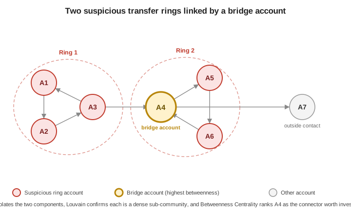
A single account rarely reveals fraud on its own; the signal is structural — a tight loop of accounts moving money between each other, plus one or two accounts that sit between that loop and the rest of the graph. Three algorithms, layered in order, surface that structure: WCC first cuts the whole transaction graph down to the connected pieces worth examining at all, Louvain then finds dense sub-communities inside each piece (a plausible laundering ring), and Betweenness Centrality ranks the accounts that bridge separate communities — the accounts most likely to be moving funds between rings rather than transacting normally within one. The first two are covered in Community Detection Algorithms and the third in Pathfinding and Centrality Algorithms.

Against the seven accounts above, WCC returns one component (everything is reachable), Louvain splits it into the two rings, and Betweenness Centrality ranks A4 highest — it sits on the only path between Ring 1, Ring 2, and the outside contact A7, exactly the account an investigator would want flagged first. See Weakly Connected Components, Louvain and Betweenness Centrality. A dedicated treatment of graph-based fraud and anti-money-laundering detection exists — see the bibliography.

Vehicle routing and delivery scheduling reduce, at the core, to weighted shortest-path search over a location graph — exactly the problem Pathfinding and Centrality Algorithms covers in depth with Dijkstra, A* and Yen’s algorithm. The only addition a logistics scenario brings is framing: the source node is a depot, the target is a delivery address, and the weight is distance, drive time, or a cost blend of both.

When the location graph carries real latitude/longitude properties, A* reaches the same optimal route while visiting fewer nodes on a large, geographically spread network, and Yen’s algorithm returns several ranked alternative routes instead of only the single best one — useful for offering a backup route or avoiding a closed road without recomputing from scratch. See Dijkstra Source-Target and A* Shortest Path.

Know-your-customer (KYC) and identity-and-access-management pipelines routinely ingest the same real-world person or account more than once, through different onboarding channels, spellings, or upstream systems. Deduplicating that graph is a two-step process: a Cypher query flags candidate duplicates by some blocking key (a normalized name plus date of birth, here), and apoc.refactor.mergeNodes — covered in APOC and the Extension Ecosystem — then folds each confirmed duplicate pair into a single node, combining their properties and re-pointing every relationship instead of leaving orphaned duplicate identities behind.

A blocking key this loose still needs a human or a scoring model in the loop before merging in production — treat the query above as the candidate-generation step, not the final decision. See apoc.refactor.mergeNodes. A dedicated treatment of entity resolution over graphs exists — see the bibliography.

Service-dependency graphs answer three closely related but distinct questions, each needing a different technique over the same :Service-[:DEPENDS_ON]-:Service graph.

Blast radius. Given a service that just started failing, which other services will eventually break? That is every service that transitively depends on it — a variable-length traversal followed upstream:

Single points of failure. The same Betweenness Centrality used to find bridge accounts above finds bridge services: the service with the highest score sits on the most dependency paths and is the one outage that would fragment the architecture the most.

Dependency-cycle validation. A healthy dependency graph should be acyclic; a cycle means two or more services depend on each other, directly or indirectly, and neither can safely start, deploy, or roll back independently. Strongly Connected Components finds exactly this: any component with more than one member is a cycle.

See Betweenness Centrality and Strongly Connected Components. A dedicated treatment of dependency-graph root-cause analysis exists — see the bibliography.

All five scenarios above are special cases of the same underlying pattern: model the domain as a property graph, project the relevant slice into GDS, and let similarity, community-detection, centrality or pathfinding algorithms surface structure that would otherwise take hand-rolled recursive queries or a separate graph-processing system to find. That is also exactly the toolbox behind general master-data-management and knowledge-graph programs — entity resolution to keep one canonical node per customer, product or organizational unit; community detection and centrality to understand how that canonical graph is actually connected; and weighted pathfinding wherever a canonical record needs a shortest or cheapest route to another. The five use cases above are simply that same toolbox applied to five concrete business questions.

See also Graph Data Science Fundamentals for the graph-projection groundwork every example on this page builds on.