Points, Lines and Planes
| This documentation was generated with the assistance of AI. Please report any inaccuracies. |
Points, lines and planes are the basic loci of irurueta-geometry, all expressed in homogeneous
coordinates so that projective operations (incidence, join, meet, transformation) reduce to linear algebra.
This page covers Point2D/Point3D, Line2D/Line3D and Plane, the duality that links them, and the two
special loci that organize the rest of projective geometry: the plane at infinity and the line at
infinity.
Points: homogeneous vs. inhomogeneous coordinates
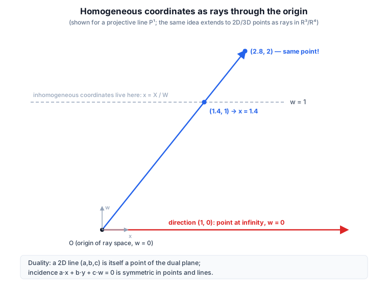
A Point<P> interface defines the dimension-agnostic contract (getDimensions(),
getInhomogeneousCoordinate(dim), distanceTo). Point2D and Point3D are abstract classes implementing it,
each with two concrete coordinate representations:
| Class | Representation | Notes |
|---|---|---|
|
|
A point at infinity has |
|
|
Equivalent to the homogeneous form with |
|
|
Same idea, one dimension up. |
|
|
Same idea, one dimension up. |
As the library’s own javadoc puts it: homogeneous points are better suited for far distances or numerical
work, while inhomogeneous points are better suited for Euclidean distance computations. toHomogeneous()/
toInhomogeneous() convert between the two freely (except that a homogeneous point at infinity has no finite
inhomogeneous equivalent). Two homogeneous points are considered equal if they agree up to a scale factor,
including sign — (x,y,w) and (-x,-y,-w) represent the same point. This is exactly the homogeneous point
of Irurueta’s thesis, §1.2.1-1.2.2 (printed pp. 2,
PDF pp. 14): a point
m = (x, y, w) converts to inhomogeneous coordinates as , and because m is only
defined up to a non-zero scale , w can always be normalized to 1 — except when w = 0,
which is precisely the case of a point at infinity.
Lines and the 2D point-line duality
Line2D stores homogeneous coefficients (a, b, c) for , with convenience
accessors for slope, y-intercept and angle.
The projective line and its duality with points
A line through a fixed point with slope can be written , which rearranges into homogeneous form as . Writing the point as and the line as , this is exactly the incidence relation
Both m and l are 3-component homogeneous vectors, but they play structurally opposite roles: a fixed l
describes the set of points lying on a line, while a fixed m describes the set of lines passing through
a point (its pencil). This symmetry is the point-line duality of
(PHD, §1.2.3, eq. 1.5-1.7, printed pp. 3,
PDF p. 15).
Duality also gives the join/meet operations their concrete cross-product form. The line through two points
m1, m2, and dually, the point where two lines l1, l2 intersect, are:
where is the standard 3-vector cross product, equivalently written as
using the skew-symmetric matrix
of a vector
(PHD, §1.2.3, eq. 1.8-1.9, printed pp. 3,
PDF pp. 15-16). This is the
"projective generalization of a cross product" that Line2D.setParametersFromPairOfPoints and
Line2D.intersection compute numerically (see Shared operations: incidence, join, meet).
Signed point-to-line distance
Because mT·l vanishes exactly for points on the line, it is proportional to the perpendicular
(signed) Euclidean distance between an arbitrary point and the line — a fact the library exposes directly as
Line2D.signedDistance(Point2D) (Line2D.java:460):
where . The sign indicates which side of the line the point lies on, according to the line’s own orientation. The full derivation (project onto the line’s director vector , then eliminate the unknown point on the line via ) is given as Proof 1.1 in PHD, §1.2.4, eq. 1.10-1.23, printed pp. 4-6, PDF pp. 16-18 — the same "dot product with the line coefficients" pattern used throughout this page for incidence testing.
Lines in 3D
Line3D is not stored as Plücker coordinates or as two points + direction: it is represented as the
intersection of two Plane objects (plane1, plane2). A point lies on the line iff it lies on both
planes; the line’s direction is recovered as the cross product of the two planes' normal vectors, and
Line3D.getDistance(Point3D) (Line3D.java:239) computes the shortest distance to a point via its closest
point on the line. This mirrors the null-space/span representation of a 3D line described in
HZ, §3.2.2 (pp. 68-70): a line is the intersection of the pencil of
planes through it, exactly as Line3D models it, rather than the Plücker-matrix or Plücker-coordinate
alternatives HZ also surveys for the same object.
Planes and the 3D point-plane duality
Plane stores homogeneous coefficients (a, b, c, d) for . Construction
options mirror the point/line "join" pattern: from three points (SVD null-space of the 3×4 coordinate
matrix), from a point plus two in-plane vectors (cross product), or from a point plus a normal vector.
The plane equation itself follows from the same linear-dependency argument as the 2D line: any point M
coplanar with three points M1, M2, M3 is a linear combination of them, so the 4×4 matrix
[M, M1, M2, M3] is singular. Expanding its determinant by Laplace’s formula along the column of M yields
, i.e. the plane’s homogeneous coefficients are exactly the
signed 3×3 minors of the other three points' coordinates
(PHD, §1.3.3, eq. 1.68-1.73, printed pp. 13-14,
PDF pp. 25-26). By analogy
with the 2D case, the point-plane incidence relation
is the 3D point-plane duality (PHD, §1.3.4, eq. 1.74, printed p. 14,
PDF p. 26): a fixed plane describes the points lying on it, a fixed point M describes the pencil
of planes through it. HZ, §3.2.1 (pp. 66-67) develops the same
relation as and adds the fact that, unlike 2D where points and lines are the only dual
pair, lines in are self-dual: a line is equally well defined as the join of two
points or the intersection of two planes, which is precisely why Line3D above is represented as two Plane
instances rather than needing a distinct dual type.
Plane.createCanonicalPlaneAtInfinity() / Plane.setAsCanonicalPlaneAtInfinity(Plane)
(Plane.java:860, Plane.java:873) return/set (a=0, b=0, c=0, d=1), normalized=true — the plane dual to
all points at infinity. The rest of this page is about that plane and its 2D counterpart, the line at infinity.
The plane at infinity and the line at infinity
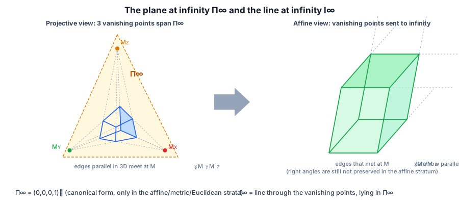
A homogeneous 3D point (X, Y, Z, W) is a point at infinity exactly when W = 0; the locus of all such points
is the plane at infinity, . Applying the point-plane duality above, its canonical
homogeneous coordinates are
(PHD, §1.4.1.1, eq. 1.118, printed p. 23,
PDF pp. 34-35; matches
HZ, §3.5, p. 80). This canonical form, however, is only guaranteed
in the affine stratum and above — it is exactly the row (0,0,0,1) that a 4×4 projective
transformation H leaves fixed if and only if H is an affinity
(HZ, Result 3.7, §3.5, p. 80). Under a general projective
transformation, moves to wherever the transformation’s last row sends it, so in an
arbitrary projective frame "the plane at infinity can be anywhere"
(PHD, §1.4.1.1, printed p. 23,
PDF p. 35). The consequence for
reconstruction pipelines is that upgrading a projective reconstruction to an affine one is exactly the problem
of identifying which plane, in the frame at hand, is playing the role of — and only
then re-expressing coordinates so it takes on its canonical form. Transformations covers that
upgrade path (and the fuller affine/metric/Euclidean stratification) in detail; this page is only concerned
with what the plane at infinity is and how to recognize it.
In practice, is identified from the image using vanishing points: because parallel
lines only meet at infinity, any three vanishing points corresponding to three independent directions in the
scene determine three points on , and hence the plane itself
(PHD, fig. 1.9, §1.4.1.1, printed p. 22-23,
PDF pp. 34-35). The
plane-at-infinity.svg diagram above shows this: in the arbitrary projective view (left) three vanishing
points mark where each family of parallel edges of the cube converges, and together
they span ; in the affine view (right) those same edges have become parallel and their
vanishing points have receded to infinity.
The line at infinity, — informally, the horizon — is the 2D analogue: it is the
intersection of with any given scene plane, or equivalently the set of vanishing points
of all directions lying in that plane. Because any two parallel planes intersect only on
, their common line lies on and is the line at infinity of either
plane’s own orientation — it depends only on the orientation of the plane, not on its position
(PHD, §1.4.1.2, fig. 1.10, printed p. 23,
PDF p. 35). This is the
projective-geometry meaning behind Line2D.createCanonicalLineAtInfinity() /
Line2D.setAsCanonicalLineAtInfinity(Line2D) (Line2D.java:789, Line2D.java:802): they return/set
(a=0, b=0, c=1), the line dual to every 2D point with w = 0, i.e. every direction rather than location.
There is no dedicated PlaneAtInfinity or LineAtInfinity class in the library — the concept is captured
entirely by these two pairs of static factory methods, one per dimension.
The following snippet illustrates the asymmetry Result 3.7 predicts: an affine transformation (here, a pure
translation) leaves the canonical plane at infinity fixed, while a general projective transformation (one with
a non-trivial last row) moves it away from (0,0,0,1):
final var pi = Plane.createCanonicalPlaneAtInfinity(); // (0, 0, 0, 1)

// an affine transformation: linear part + translation, last row (0,0,0,1)
final var affine = new Matrix(4, 4);
affine.setElementAt(0, 0, 1.0);
affine.setElementAt(1, 1, 1.0);
affine.setElementAt(2, 2, 1.0);
affine.setElementAt(0, 3, 5.0);   // translation
affine.setElementAt(1, 3, -2.0);
affine.setElementAt(2, 3, 3.0);
affine.setElementAt(3, 3, 1.0);

// planes transform with the inverse-transpose of the point transformation
// (see xref:transformations.adoc[]); the plane at infinity stays canonical
final var piAffine = /* apply inverse-transpose of affine to pi */ pi;
// piAffine still equals (0, 0, 0, 1) up to scale

// a general projective transformation: non-trivial last row
final var projective = new Matrix(4, 4);
projective.setElementAt(0, 0, 1.0);
projective.setElementAt(1, 1, 1.0);
projective.setElementAt(2, 2, 1.0);
projective.setElementAt(3, 0, 0.001); // breaks affinity: last row is not (0,0,0,1)
projective.setElementAt(3, 3, 1.0);

// piProjective no longer equals the canonical plane at infinity
And the join/meet pattern applied to the canonical line at infinity in 2D — confirming that only points with
w = 0 are incident with it:
final var lineAtInfinity = Line2D.createCanonicalLineAtInfinity(); // (0, 0, 1)

final var direction = new HomogeneousPoint2D(1.0, 2.0, 0.0);  // w = 0: a direction
final var location = new HomogeneousPoint2D(1.0, 2.0, 1.0);   // w = 1: a finite point

lineAtInfinity.isLocus(direction); // true  -- directions lie on l_infinity
lineAtInfinity.isLocus(location);  // false -- finite points do not
Shared operations: incidence, join, meet
The same three linear-algebra patterns recur across points/lines/planes:
| Operation | How it’s computed |
|---|---|
Incidence ( |
dot product of a point’s homogeneous coordinates with the line/plane coefficients, compared to a threshold
(e.g. |
Join (points → line/plane) |
|
Meet (lines/planes → point) |
|
Both operations reduce to finding the null-space of a small matrix via Singular Value Decomposition
(com.irurueta.algebra.SingularValueDecomposer, used internally by all four methods above): a point/line/plane
is incident with every row of the stacked matrix exactly when it lies in that matrix’s null-space, and for a
rank-deficient matrix built from 2 points (2D join) or 3 points (3D join) that null-space is one-dimensional — the sought line or plane, up to scale. This is the general numerical technique behind the closed-form cross
product, described in Numerical Recipes, §2.6, "Singular Value
Decomposition" and §2.6.1, "Range, Nullspace, and All That" (pp. 65, 67), and, for the exact same construction
applied to points/planes/lines in , in HZ,
§3.2.1 (eq. 3.3-3.5, pp. 66-68).
Join and meet being the same numerical operation (a null-space computation) applied to different inputs is the
computational signature of point-line duality in 2D, and point-plane duality in 3D — even though the
code itself never uses the word "dual" in these six classes. The word is used explicitly one level up, for
conic/dual-conic and quadric/dual-quadric (see Conics and Quadrics), which realize the same point/line
and point/plane duality concretely through DualConic/DualQuadric.
References
-
Irurueta, A., Fixed Scene 3D Reconstruction for Mobile Applications (PhD thesis) — §1.2.1-1.2.2 (printed p. 2, PDF p. 14) for homogeneous vs. inhomogeneous 2D coordinates; §1.2.3, eq. 1.5-1.9 (printed p. 3, PDF p. 15) for the point-line duality and the cross-product join/meet; §1.2.4, eq. 1.10-1.23 and Proof 1.1 (printed pp. 4-6, PDF pp. 16-18) for the signed point-to-line distance underlying
Line2D.signedDistance; §1.3.3, eq. 1.68-1.73 (printed pp. 13-14, PDF pp. 25-26) for the plane equation via the 4×4 determinant/Laplace expansion; §1.3.4, eq. 1.74 (printed p. 14, PDF p. 26) for the 3D point-plane duality; §1.4.1.1, eq. 1.118 and fig. 1.9 (printed pp. 22-23, PDF pp. 34-35) for the plane at infinity and its identification via vanishing points; §1.4.1.2 and fig. 1.10 (printed p. 23, PDF p. 35) for the line at infinity; §1.4.2, eq. 1.119-1.127 (printed pp. 24-25, PDF pp. 36-37) for why the plane at infinity is fixed by affine transformations. -
Hartley & Zisserman, Multiple View Geometry in Computer Vision, 2nd ed. — chapter 2 for the analogous 2D point-line duality and join/meet in ; §3.2.1-3.2.2 (pp. 66-70) for point-plane duality, the self-duality of lines in , and the null-space/span line representation
Line3Dmirrors; §3.5, Result 3.7 (p. 80) for the plane at infinity and its invariance under exactly the affine group; §3.6, eq. 3.21-3.23 and Result 3.9 (pp. 81-82) for the absolute conic that lies on the plane at infinity (see Conics and Quadrics and Transformations). -
Press, Teukolsky, Vetterling & Flannery, Numerical Recipes: The Art of Scientific Computing, 3rd ed. — §2.6 and §2.6.1 (pp. 65, 67) for Singular Value Decomposition and its null-space/range interpretation, the general numerical technique behind every join/meet computation on this page.
Related pages
-
Transformations — the full projective/affine/metric/Euclidean stratification, the inverse-transpose transformation rule for lines and planes, and how the plane at infinity is upgraded to its canonical position.
-
Conics and Quadrics — second-degree curves/surfaces built on top of points, and their duals, including the absolute conic that lives on the plane at infinity.
-
Triangles and Polygons — composite entities built from points.
-
Pinhole Camera — projecting 3D points/lines/planes into a 2D image.