Downhill Simplex Method (Nelder-Mead)
| This documentation was generated with the assistance of AI. Please report any inaccuracies. |
The downhill simplex method is a self-contained strategy for minimizing a function of several variables using
only function evaluations — no derivatives, and no one-dimensional line minimization as a building block
(unlike every other multi-variable optimizer in this package). It is slow compared to those alternatives, but
geometrically simple and remarkably robust. It is described in Press et al.,
2007, Section 10.5 (page 502), and implemented as SimplexMultiOptimizer in the
com.irurueta.numerical.optimization package.
The simplex
In dimensions, a simplex is the figure formed by vertices and all the line segments, faces, etc. connecting them — a triangle in 2D, a (not necessarily regular) tetrahedron in 3D. Given a starting point and a characteristic length scale (or a separate scale per direction), the other vertices are:
where are the unit vectors. Unlike one-dimensional minimization, there is no way to bracket a multidimensional minimum — the simplex method instead has to make its own way downhill from this initial guess, wherever that leads.
Reflect, expand, contract, shrink
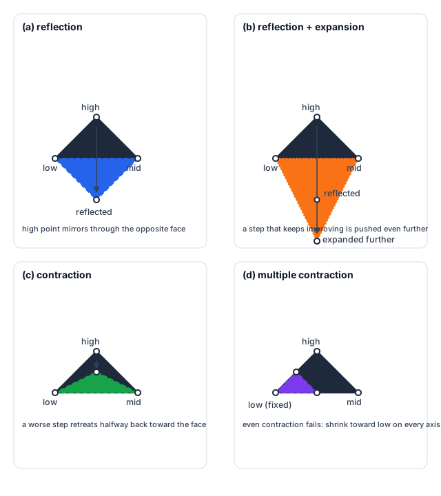
Each step identifies the simplex’s highest (worst), second-highest, and lowest (best) vertices by function value, then tries to replace the worst one by reflecting it through the centroid of all the others:
with for a plain reflection. Depending on how that reflected point compares to the rest of the simplex, one of four outcomes follows:
-
Reflection improves on the best point — the simplex is trying something good; push further with an expansion ( ) in the same direction, keeping whichever of the reflected or expanded point is better.
-
Reflection is worse than the second-highest point — look for a nearer intermediate point instead via a one-dimensional contraction ( ) toward the centroid.
-
Even the contracted point fails to improve — the simplex may be trying to "pass through the eye of a needle"; shrink it around its best (lowest) vertex, halving the distance from every other vertex to that one.
-
Otherwise — the plain reflected point is accepted as-is.
Reflections and expansions conserve the simplex’s volume (and hence its nondegeneracy); contractions and shrinks reduce it, letting the simplex "ooze" down a valley floor or squeeze through a narrow passage.
Termination and restarts
With no bracket to shrink, convergence is instead judged from one full step (one reflect/expand/contract/shrink cycle) to the next: this package stops once the fractional range between the highest and lowest function values in the simplex, , drops below the configured tolerance. A single anomalous step that makes no progress can fool this test, so Press et al., 2007 recommends restarting the method at the point it claims is a minimum — reinitializing a fresh simplex there — cheap to do, since it already converged to that point once.
Library implementation
SimplexMultiOptimizer extends MultiOptimizer directly (not the line-search-based LineMultiOptimizer
hierarchy used by every other multi-variable optimizer here, since this method needs no 1D line
minimization). The initial simplex can be supplied three ways:
-
setSimplex(startPoint, delta)— a single length scale used identically along every coordinate direction. -
setSimplex(startPoint, deltas)— a separate length scale per coordinate direction. -
setSimplex(Matrix)— the full matrix of vertex coordinates directly.
Convergence is controlled by getTolerance() / setTolerance(double) (fractional tolerance on the function
value, default 3e-8); up to NMAX = 5000 function evaluations are allowed before the optimizer reports
failure. After minimize(), in addition to the usual getResult() / getEvaluationAtResult(),
getEvaluationsAtSimplex() returns the function values at every vertex of the final simplex.
| Press et al., 2007 positions this method as the right tool when "get something working quickly" matters more than raw efficiency, for a problem cheap enough that many function evaluations are not a concern. Powell’s method or the quasi-Newton method (with numerically estimated gradients) is almost always faster once that efficiency starts to matter. |
Example
final var listener = new MultiDimensionFunctionEvaluatorListener() {
    @Override
    public double evaluate(final double[] point) {
        final var dx = point[0] - 1.0;
        final var dy = point[1] + 2.0;
        return dx * dx + dy * dy;
    }
};

final var startPoint = new double[]{0.0, 0.0};
final var optimizer = new SimplexMultiOptimizer(listener, startPoint, 1.0, 3e-8);
optimizer.minimize();

final var xmin = optimizer.getResult();          // approximately [1.0, -2.0]
final var fmin = optimizer.getEvaluationAtResult(); // approximately 0.0| Class | Javadoc | Source |
|---|---|---|
|
||
|