Levenberg-Marquardt Fitting Algorithm
| This documentation was generated with the assistance of AI. Please report any inaccuracies. |
The Levenberg-Marquardt method is an iterative algorithm for fitting a model that depends nonlinearly on its
parameters to a set of data points, in the least-squares sense. It is the algorithm behind
LevenbergMarquardtSingleDimensionFitter, LevenbergMarquardtMultiDimensionFitter, and
LevenbergMarquardtMultiVariateFitter in the com.irurueta.numerical.fitting package, and is described in
Press et al., 2007, Section 15.5.2 (page 801).
Problem statement
Given a model with unknown parameters , and measured data points with standard deviations , the goal is to find the parameters that minimize the chi-square merit function:
Unlike the linear least-squares fitters, this cannot be solved in one step: the model’s dependence on is nonlinear, so the minimization has to proceed iteratively from an initial guess.
Gradient, curvature, and two extreme strategies
Close enough to the minimum, is well approximated by a quadratic form, and the parameters that minimize it can be reached in a single Newton step using the gradient and the Hessian (the curvature matrix) of . Following the conventional definitions:
Expanding these from the definition of gives:
(a second-derivative term is dropped from — it tends to cancel out over well-behaved residuals and including it can destabilize the fit in the presence of outliers or a poor model).
The Newton step is the solution of the linear system:
This works well near the minimum, but can badly overshoot far from it. Far from the minimum, a small step down the gradient (steepest descent) is safer:
but there is no good way to know what "constant" should be.
Marquardt’s two insights
Marquardt’s contribution was a way to interpolate smoothly between these two strategies:
-
The diagonal element has exactly the right dimensions to set the scale of the steepest-descent step, giving for a dimensionless damping factor .
-
Both strategies can be expressed as a single linear system by defining an augmented curvature matrix :
When is large, is diagonally dominant and the system reduces to the steepest-descent step; as it reduces to the Newton (inverse-Hessian) step. Every iteration solves the same augmented system — only changes.
Algorithm
Given an initial guess for :
Stated as a recipe:
-
Compute .
-
Pick a modest value for (e.g. ).
-
Solve the augmented linear system for and evaluate .
-
If the trial is worse ( ), increase by a factor of 10 and go back to step 3.
-
If the trial is better, decrease by a factor of 10, accept , and go back to step 3.
-
Stop once has decreased by a negligible amount for a few consecutive successful iterations (iterating to machine precision is wasteful, since the minimum is only a statistical estimate). Do one final pass with and compute the covariance matrix of the fitted parameters:
Library implementation
The three fitter classes share this structure; they differ only in the shape of the input/output data and of the evaluator listener they require:
| Class | Model | Evaluator interface |
|---|---|---|
|
, scalar |
|
|
, vector-valued |
|
|
, vector-valued and |
|
Each evaluator is responsible for two things, mirroring Fitmrq’s `funks callback in
Press et al., 2007: supplying the initial parameter guess
(createInitialParametersArray()), and evaluating both the model and its derivatives/Jacobian with respect to
at a given sample (evaluate(…)).
After fit() completes, each fitter exposes:
-
getA()— the fitted parameters . -
getCovar()— the covariance matrix of the fitted parameters. -
getAlpha()— the curvature matrix at the solution. -
getChisq()— the final value;getChisqDegreesOfFreedom(),getP(), andgetQ()turn it into a goodness-of-fit probability via the chi-square distribution. -
getMse()— mean square error of the residuals.
hold(i, val) / free(i) let selected parameters be fixed at a known value during fitting (they are excluded
from but still appear in the model), matching Fitmrq’s `hold/free methods.
Convergence is tuned via setNdone(int) (consecutive negligible-improvement iterations before stopping,
default 4), setItmax(int) (maximum iterations, default 5000), and setTol(double) (the "negligible" threshold
on , default 1e-3).
By default (setCovarianceAdjusted(true)) the fitters additionally rescale the raw
covariance using the input samples' Jacobians and standard deviations
( ) to produce a covariance on the true scale of the problem, as discussed
in Press et al., 2007, Section 15.6 (page 812).
|
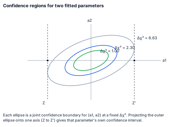
The covariance matrix is what makes this picture possible: its diagonal gives each parameter’s own variance, directly usable for -style intervals, while the full matrix (diagonal and off-diagonal terms) traces out the joint confidence ellipse shown above for any pair of parameters — a strictly larger region than treating the two parameters as independent would suggest, whenever they are correlated.
Example
Fitting a single Gaussian — the same example
model used in Press et al., 2007, Section 15.5.3 — to data x, y, sigma:
final var evaluator = new LevenbergMarquardtSingleDimensionFunctionEvaluator() {
    @Override
    public double[] createInitialParametersArray() {
        // initial guess: amplitude, center, width
        return new double[]{1.0, 0.0, 1.0};
    }

    @Override
    public double evaluate(final int i, final double point, final double[] params,
                            final double[] derivatives) {
        final var amplitude = params[0];
        final var center = params[1];
        final var width = params[2];
        final var arg = (point - center) / width;
        final var exponential = Math.exp(-arg * arg);
        final var factor = 2.0 * amplitude * exponential * arg;

        derivatives[0] = exponential;
        derivatives[1] = factor / width;
        derivatives[2] = factor * arg / width;

        return amplitude * exponential;
    }
};

final var fitter = new LevenbergMarquardtSingleDimensionFitter(evaluator, x, y, sigma);
fitter.fit();

final var params = fitter.getA();          // fitted [amplitude, center, width]
final var covariance = fitter.getCovar();   // covariance matrix of the parameters
final var chiSq = fitter.getChisq(); // goodness-of-fit statistic| Class | Javadoc | Source |
|---|---|---|
|
||
|
When to use it
Levenberg-Marquardt requires a plausible initial guess and only finds a local minimum of — it has no special ability to locate the global minimum among several local ones. It works very well in practice once a reasonable starting point is available, which is why it is normally used as the "endgame" refinement step, possibly preceded by a cruder, problem-specific method to get into the right basin of convergence. See Press et al., 2007, Section 15.5.4, for pointers to more advanced alternatives (e.g. full-Newton or trust-region variants) when Levenberg-Marquardt converges too slowly or to the wrong minimum.