Conjugate Gradient Methods
| This documentation was generated with the assistance of AI. Please report any inaccuracies. |
When a function’s gradient is available, it carries far more information per evaluation than a bare function
value — enough, used wisely, to build up a set of conjugate
directions in only line minimizations instead of . Conjugate gradient methods do
exactly this, using only storage. This package implements the Fletcher-Reeves and Polak-Ribière
variants, described in Press et al., 2007, Section 10.8 (page 515), as
ConjugateGradientMultiOptimizer (numerically estimated or user-supplied gradient, non-derivative line search)
and DerivativeConjugateGradientMultiOptimizer (derivative-aware line search) in the
com.irurueta.numerical.optimization package.
Why not just follow the gradient downhill?
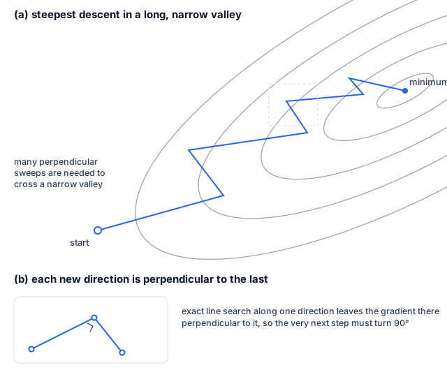
The obvious approach — repeatedly line-minimize along the local downhill gradient , the steepest descent method — has the same problem as minimizing along the coordinate axes one at a time: the new gradient at any line minimum is, by construction, perpendicular to the direction just traversed. In a long, narrow valley this forces a sequence of right-angle turns, taking many small steps to reach the valley floor instead of running straight down it.
Constructing conjugate directions from gradients alone
For the local quadratic approximation , a remarkable fact makes this tractable without ever forming or storing the Hessian : if , and is the result of line- minimizing from along a direction , then setting gives exactly the same vector that the classical conjugate-gradient recurrence for linear systems would have constructed using directly:
So a sequence of mutually conjugate search directions can be built using nothing but gradient evaluations and line minimizations — no Hessian required, no storage. The two variants implemented here differ only in the formula used for :
The two formulas are algebraically equal for an exact quadratic form, but real functions are never exactly
quadratic. Polak-Ribière tends to handle the transition more gracefully once the method has essentially
converged and is running out of useful conjugate structure: it naturally resets the search direction back
toward the local gradient, effectively restarting the method — which is why this package uses it as the
default (usePolakRibiere = true), while still allowing Fletcher-Reeves via a constructor flag.
Two line-search strategies
Both classes share this same direction-update logic, differing only in how each 1D sub-problem is solved:
-
ConjugateGradientMultiOptimizerbuilds onLineMultiOptimizer— the same accurate, Brent-based line search that Powell’s method uses, ignoring the gradient during the 1D search itself. -
DerivativeConjugateGradientMultiOptimizerbuilds onDerivativeLineMultiOptimizer, which drivesDerivativeBrentSingleOptimizerinstead — using the gradient’s projection along the search direction to speed up each line minimization too.
Library implementation
Both classes require a GradientFunctionEvaluatorListener in addition to the usual
MultiDimensionFunctionEvaluatorListener:
| Class | Line search |
|---|---|
|
Non-derivative ( |
|
Derivative-aware ( |
Both share:
-
setGradientListener(…)— supplies ; if an analytic gradient is not available, wrap a numericalGradientEstimatorin this listener instead. -
isPolakRibiereEnabled()/setUsePolakRibiere(boolean)— selects between the two variants (default: Polak-Ribière). -
getTolerance()/setTolerance(double)— the fractional tolerance on the function value; default3e-8. -
getIterations()— the number of iterations actually used, afterminimize()completes.
Convergence is checked three ways each iteration: the relative decrease in the function value, the (scaled)
maximum gradient component, and an exact zero gradient — whichever triggers first ends the search. Up to
ITMAX = 200 iterations are attempted.
| Press et al., 2007 considers quasi-Newton methods to generally dominate conjugate gradient methods when the extra storage they require is affordable — but conjugate gradient remains the right choice when memory is at a premium for large . |
Example
final var listener = new MultiDimensionFunctionEvaluatorListener() {
    @Override
    public double evaluate(final double[] point) {
        final var dx = point[0] - 1.0;
        final var dy = point[1] + 2.0;
        return dx * dx + dy * dy;
    }
};
final var gradientListener = new GradientFunctionEvaluatorListener() {
    @Override
    public void evaluateGradient(final double[] params, final double[] result) {
        result[0] = 2.0 * (params[0] - 1.0);
        result[1] = 2.0 * (params[1] + 2.0);
    }
};

final var optimizer = new ConjugateGradientMultiOptimizer(
        listener, gradientListener, new double[]{0.0, 0.0}, 3e-8, true);
optimizer.minimize();

final var xmin = optimizer.getResult();          // approximately [1.0, -2.0]
final var fmin = optimizer.getEvaluationAtResult(); // approximately 0.0| Class | Javadoc | Source |
|---|---|---|
|
||
|
||
|