Polynomial Interpolation
| This documentation was generated with the assistance of AI. Please report any inaccuracies. |
Given a table of points , polynomial interpolation estimates at an arbitrary
by drawing the unique polynomial of degree through the tabulated points nearest
. It is described in Press et al., 2007, Sections 3.1 (page 114,
searching an ordered table) and 3.2 (page 118, polynomial interpolation), and implemented as
LinearInterpolator and PolynomialInterpolator in the com.irurueta.numerical.interpolation package, both
sharing the table-search machinery of the BaseInterpolator base class.
Searching an ordered table
Before interpolating, every 1D interpolator in this package first needs to find which consecutive
tabulated abscissas to center the interpolation on. BaseInterpolator provides two strategies for this:
-
locate(x)— plain bisection search, . -
hunt(x)— starts from the position found by the previous call and hops outward in exponentially growing steps (1, 2, 4, …) until it brackets , then bisects within that bracket.
interpolate(x) automatically picks whichever of the two is likely to win, based on whether the two most
recent calls landed close together in the table:
hunt is faster than locate when consecutive calls ask for nearby values of — a common pattern,
e.g. when the interpolator is called from the right-hand side of an ODE integrator stepping steadily forward —
but can be up to twice as slow as locate in the worst case, if the guess is far from where actually
falls.
Linear interpolation
The simplest case, using just the points bracketing :
LinearInterpolator implements exactly this formula, with no configurable order.
Polynomial interpolation via Neville’s algorithm
For points, the unique interpolating polynomial of degree is given explicitly by Lagrange’s classical formula, but evaluating it directly is both awkward to code and gives no error estimate. Neville’s algorithm builds the same polynomial recursively instead, via a triangular tableau of partial polynomials — the value at of the unique polynomial through consecutive tabulated points. Each entry is built from its two "parents" in the previous column:
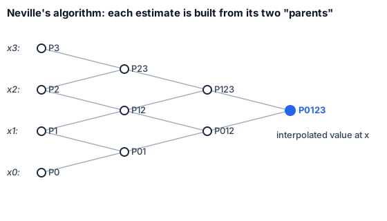
Tracking only the small differences between a column’s parents and daughters — rather than the full values — gives a numerically better-behaved recurrence for the correction terms and :
At each stage, the accumulated answer is any starting plus a chain of 's and/or 's following the "straightest line" path through the tableau toward its apex — which also keeps the partial approximations centered on . The size of the last correction added is a natural, if informal, error estimate for the whole interpolation.
Library implementation
Both classes extend BaseInterpolator and expose the same interpolate(x) entry point:
| Class | Order | Notes |
|---|---|---|
|
Fixed at |
No error estimate (the model is exact between adjacent points by construction). |
|
Configurable (constructor parameter, or all points by default) |
|
Increasing does not always improve accuracy — quite the opposite for equally-spaced abscissas,
where high-order polynomial interpolation is notoriously ill-conditioned and prone to wild oscillation between
tabulated points. Prefer a small, local (3 or 4 points is often plenty, rarely more than 5 or 6)
centered on , rather than constructing PolynomialInterpolator with its default of all the points in
the table.
|