Linear Least-Squares Fitting Algorithm
| This documentation was generated with the assistance of AI. Please report any inaccuracies. |
Linear least-squares fitting estimates the coefficients of a model that is a linear combination of arbitrary,
fixed basis functions, by directly solving the normal equations of the least-squares problem. It is the
algorithm behind SimpleSingleDimensionLinearFitter (and its multi-dimensional counterpart,
MultiDimensionLinearFitter’s own simple implementation) in the `com.irurueta.numerical.fitting package, and
is described in Press et al., 2007, Section 15.4.1 (page 789).
Problem statement
Unlike Levenberg-Marquardt fitting, here the model does not need to be a straight line or even a polynomial — only linear in its parameters. Given arbitrary, fixed basis functions (e.g. for a polynomial, or sines and cosines for a Fourier series), the model is:
and the parameters are chosen to minimize the same chi-square merit
function used throughout the fitting package:
where is the known (or assumed constant) measurement error of each data point. Because is quadratic in , its minimum can be found directly, in one step, rather than iteratively.
Design matrix and normal equations
Define the design matrix and the length- vector from the basis functions and the data:
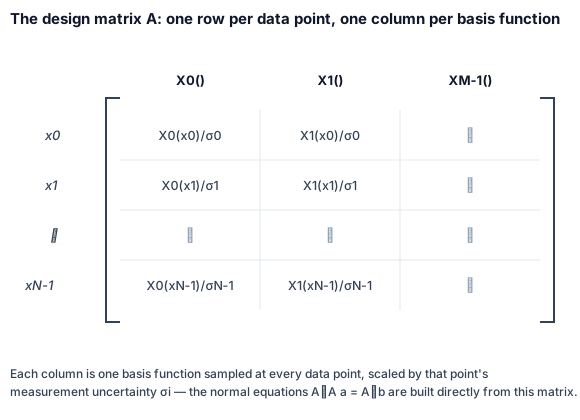
Setting for every parameter gives the normal equations:
with
Solving this linear system for (by Gauss-Jordan elimination, LU decomposition, or Cholesky decomposition, since is symmetric positive-definite) gives the best-fit parameters directly — no initial guess or iteration required.
Covariance of the fitted parameters
The same Gauss-Jordan elimination that solves can be run in a form that also produces as a side effect, at essentially no extra cost. This inverse is the covariance matrix of the fit:
Its diagonal elements are the variances of the fitted parameters, , and its off-diagonal elements are the covariances between and .
Algorithm
Because the fit is a single linear solve, there is no damping factor, no convergence tolerance, and no maximum-iteration count to configure — the closed-form solution is exact up to the numerical stability of the linear solver.
Freezing parameters
As with the Levenberg-Marquardt fitters, individual parameters can be held fixed at a known value instead of
being estimated (e.g. because they come from theory or from a previous experiment) via hold(i, val) /
free(i), mirroring Fitlin’s `hold/free methods. Held parameters are subtracted out of before
the remaining, free parameters are solved for, and they are reported back with zero variance and covariance.
Library implementation
SimpleSingleDimensionLinearFitter extends SingleDimensionLinearFitter, which in turn extends
SingleDimensionFitter. The evaluator supplied to it, LinearFitterSingleDimensionFunctionEvaluator, has a
narrower contract than the Levenberg-Marquardt evaluators — it only needs to report the basis functions'
values, not any derivative:
-
createResultArray()— allocates the array of length that will hold one evaluation. -
evaluate(double point, double[] result)— fillsresultwith atpoint.
After fit() completes:
-
getA()— the fitted parameters . -
getCovar()— the covariance matrix of the fitted parameters. -
getChisq()— the final value.
Solving the normal equations directly is susceptible to roundoff error, because the condition number of
is the square of the condition number of . When the basis
functions are close to degenerate — a common occurrence — prefer the SVD-based
SvdSingleDimensionLinearFitter / SvdMultiDimensionLinearFitter (Press et al.,
2007, Section 15.4.2, page 794) instead, which solves the same problem in a way that cannot fail even when
alpha is singular. SimpleSingleDimensionLinearFitter is best reserved for well-conditioned basis sets, where
it is cheaper.
|
Example
Fitting a cubic polynomial to data x, y, sigma — the same
cubicfit example used in Press et al., 2007:
final var evaluator = new LinearFitterSingleDimensionFunctionEvaluator() {
    @Override
    public double[] createResultArray() {
        return new double[4];
    }

    @Override
    public void evaluate(final double point, final double[] result) {
        result[0] = 1.0;
        for (var i = 1; i < 4; i++) {
            result[i] = point * result[i - 1];
        }
    }
};

final var fitter = new SimpleSingleDimensionLinearFitter(evaluator, x, y, sigma);
fitter.fit();

final var params = fitter.getA();          // fitted [a0, a1, a2, a3]
final var covariance = fitter.getCovar();  // covariance matrix of the parameters
final var chiSq = fitter.getChisq(); // goodness-of-fit statistic| Class | Javadoc | Source |
|---|---|---|
|
||
|