Self-calibration
| This documentation was generated with the assistance of AI. Please report any inaccuracies. |
When a scene is reconstructed from image correspondences alone, without any known camera intrinsics, the
result lives in an arbitrary projective stratum: cameras and 3D points are only defined up to an unknown
projective transformation. Self-calibration recovers enough information about the cameras'
intrinsic parameters to upgrade that reconstruction to a metric stratum — correct up to a similarity
(scale, rotation, translation) — with no calibration object required. This page covers the two methods
irurueta-ar implements: the dual absolute quadric (recommended) and the Kruppa equations (simpler,
but more prone to degeneracies).
The absolute dual quadric and the dual image of the absolute conic
The plane at infinity and the absolute conic on it are invariant under similarity transformations but not under general projective ones; together they fully characterize the metric stratum. Their projective-invariant algebraic encoding is the absolute dual quadric , which in the metric stratum is simply
Projecting it into any view gives the dual image of the absolute conic (DIAC) : in the metric stratum this reduces to , a real symmetric, positive-definite matrix. This is the key fact self-calibration exploits both ways: estimating (or per view) recovers via a Cholesky factorization of the DIAC Irurueta, PhD thesis §5.2.
Maps to com.irurueta.ar.calibration.DualAbsoluteQuadric, DualImageOfAbsoluteConic (its Cholesky-derived
intrinsics via getIntrinsicParameters()), and ImageOfAbsoluteConic (the non-dual form, projected instead
from the absolute conic itself).
Calibration using the dual absolute quadric
Assuming some combination of zero skew, a principal point at the image origin, and unit aspect ratio (all common and reasonable for consumer cameras), the DIAC in each view reduces to — three off-diagonal zeros plus one equality constraint per view, each linear in the unknown entries of once expressed through the projective camera matrices of that (otherwise arbitrary-projective) stratum:
Stacking these across at least 3 views (the reference camera alone gives a degenerate system) yields a homogeneous linear system solved by the SVD null-space, exactly as in the fundamental matrix’s linear estimation Irurueta, PhD thesis §5.3.1. From the recovered , the focal length of each view falls out of its diagonal DIAC entry, and the plane at infinity’s direction falls out of 's last row/column — together giving the projective-to-metric transform
(using either a per-view , or the first view’s / the mean if intrinsics are assumed constant across the sequence) Irurueta, PhD thesis §5.3.1.1-5.3.1.2. Applying to every triangulated point upgrades the whole reconstruction to metric; applying upgrades the camera matrices.
Maps to com.irurueta.ar.calibration.estimators.DualAbsoluteQuadricEstimator (LMSEDualAbsoluteQuadricEstimator,
WeightedDualAbsoluteQuadricEstimator, or the robust family
{RANSAC,LMedS,MSAC,PROSAC,PROMedS}DualAbsoluteQuadricRobustEstimator following
Robust vs. non-robust estimation), with setZeroSkewness, setPrincipalPointAtOrigin, and
setFocalDistanceAspectRatioKnown controlling exactly which of the assumptions above are enforced.
Enforcing the rank-3 constraint
A general symmetric quadric has 10 independent entries, so DualAbsoluteQuadricEstimator
actually solves for the full 10-parameter vector rather than the simplified
6-parameter form shown above; the zero-skew/unit-aspect-ratio/known-principal-point assumptions only fix
which rows of the linear system look like the equations above, not the size of itself. With one
camera discarded as degenerate, each additional view still contributes the same handful of homogeneous linear
equations in , stacked into a matrix and solved through its SVD .
Because the Dual Absolute Quadric is only guaranteed to be singular (rank 3, as any real dual quadric of a
proper quadric surface must be) when the linear system leaves exactly one free scale, but a handful of views
under a partial assumption set can leave the last two singular vectors of
unconstrained, the estimator does not simply take as the answer. Instead it takes the general
solution as a linear combination , substitutes it into the requirement
, and expands this determinant into a quartic polynomial in — exactly the same companion-matrix eigenvalue technique used for the
7-point algorithm's cubic (there in 1 free parameter instead of 2, and
degree 3 instead of 4). Each real root of the quartic is evaluated and the one that best satisfies the DAQ’s
algebraic constraints is kept as the final, singularity-enforced solution. This behavior is controlled by
setSingularityEnforced (isSingularityEnforced), on by default; disabling it skips this step and simply
returns the raw SVD null-space solution, which is faster but not guaranteed to be a valid (singular) quadric.
LMSE vs. weighted solutions
Both concrete non-robust estimators solve the same linear system, but differ in how they combine more views than the strict minimum:
-
LMSEDualAbsoluteQuadricEstimatorstacks every provided camera’s equations with equal weight and, whensetLMSESolutionAllowedis enabled and more than the minimum number of cameras is supplied, takes the overdetermined least-mean-squared-error solution (the smallest-singular-value right singular vector of the full stacked ) instead of an exact minimal solution. -
WeightedDualAbsoluteQuadricEstimatorinstead accepts an explicit per-camera quality weight, sorts cameras by weight, and caps how many actually enter the linear system (DEFAULT_MAX_CAMERAS = 50). This matters once a reconstruction has accumulated far more views than are needed algebraically: rather than solving an ever-growing, equally-weighted system, only the most reliable (highest-weight) views are kept, bounding both the computational cost and the influence of poorly conditioned cameras.
The robust family ({RANSAC,LMedS,MSAC,PROSAC,PROMedS}DualAbsoluteQuadricRobustEstimator) wraps either
non-robust solver inside the same outlier-rejection loop used
everywhere else in this library, scoring each candidate DAQ by how well the other cameras (not in the current
minimal sample) satisfy its induced DIAC constraints — useful when some estimated camera matrices in the
sequence are themselves inaccurate (e.g. from a poorly resectioned view).
Estimating the image of the absolute conic from homographies
A complementary route to the same DIAC/IAC relationship uses 2D homographies instead of full camera matrices,
and is what com.irurueta.ar.calibration.estimators.ImageOfAbsoluteConicEstimator implements. Given a
homography mapping a reference plane’s points into a view, the IAC
satisfies two constraints per homography (the same ones underlying Zhang’s calibration
method):
The IAC has 5 independent entries (up to scale), so in general , i.e. at
least 3 homographies are needed. Each simplifying assumption removes one unknown and one required homography:
assuming zero skew needs only homographies, and further assuming a
principal point at the origin needs only — a single homography
suffices, controlled by the same setZeroSkewness/setPrincipalPointAtOrigin style flags as the DAQ estimator.
Once is known, intrinsics follow from a Cholesky-related factorization exactly as for its
dual, the DIAC (§"The absolute dual quadric…" above).
This is the same machinery that underlies pattern-based calibration
(where maps a known calibration pattern’s ideal points into each photographed view) — the only
difference from self-calibration is where the homographies come from: a physical pattern there, versus a
plane-induced homography between two already-reconstructed (projective) views here, or the DAQ-based
projective camera matrices above. com.irurueta.ar.calibration.estimators.LMSEImageOfAbsoluteConicEstimator and
WeightedImageOfAbsoluteConicEstimator mirror the DAQ estimator’s LMSE-vs-weighted distinction, and
{RANSAC,LMedS,MSAC,PROSAC,PROMedS}ImageOfAbsoluteConicRobustEstimator again add outlier rejection over a
larger set of homographies following Robust vs. non-robust estimation.
The Kruppa equations
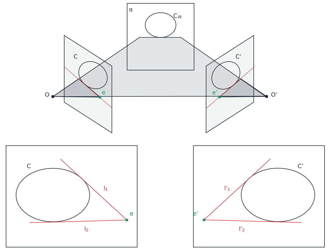
The Kruppa equations are the historically earlier self-calibration method, and only need a pair of views' fundamental matrix — no full camera matrices required. They come from epipolar tangency: the two epipolar lines from an epipole tangent to a conic map, under the epipolar geometry, to the two tangent lines from the other epipole tangent to the corresponding conic in the other view. Applying this to the absolute conic itself (so the conics become the DIACs , of each view) gives
which, substituting the SVD (so , ), reduces to the classic three-way equality relating entries of both DIACs to Irurueta, PhD thesis §5.3.2:
Under the same zero-skew/unit-aspect-ratio/known-principal-point assumptions as above, this gives enough equations to solve for the (constant) focal length from a single pair of views — fewer views than the dual absolute quadric method needs — but it only recovers the DIAC, not the plane at infinity, so it is more sensitive to degenerate configurations and is used here as a fallback rather than the default Irurueta, PhD thesis §5.3.2, §5.5.
Maps to com.irurueta.ar.calibration.estimators.KruppaDualImageOfAbsoluteConicEstimator.
Critical motion sequences
Both methods can degenerate for certain camera motions: pure rotation about a single axis, too little translation between views, or a narrow field of view all reduce the rank of the linear systems above and make the recovered / unreliable. General, wide camera motion (translation in more than one direction, varied viewing angles) avoids these critical sequences Irurueta, PhD thesis §5.4. The more assumptions you can safely make about up front (zero skew, known principal point, unit aspect ratio), the fewer free parameters remain to absorb such degeneracies.
Example
// Dual absolute quadric self-calibration from >= 3 projective cameras
var daqEstimator = DualAbsoluteQuadricEstimator.create(projectiveCameras);
daqEstimator.setZeroSkewness(true);
daqEstimator.setPrincipalPointAtOrigin(true);
daqEstimator.setFocalDistanceAspectRatioKnown(true);
DualAbsoluteQuadric daq = daqEstimator.estimate();

// Kruppa equations from a single pair of views (only needs F)
var kruppaEstimator = new KruppaDualImageOfAbsoluteConicEstimator(fundamentalMatrix);
DualImageOfAbsoluteConic diac = kruppaEstimator.estimate();
PinholeCameraIntrinsicParameters intrinsics = diac.getIntrinsicParameters();Next
See Structure from Motion for how self-calibration fits into the full reconstruction pipeline: projective reconstruction first, self-calibration second, metric reconstruction last.
References
Irurueta, PhD thesis §1.4.3, §5
Hartley & Zisserman, 2003 chapter 19 ("Auto-Calibration")
Hartley & Zisserman, 2003 §3.6-3.7 (absolute conic / dual
quadric)