RSSI-based position estimators
| This documentation was generated with the assistance of AI. Please report any inaccuracies. |
The com.irurueta.navigation.indoor.position package estimates a device’s position from received signal
strength (RSSI) readings, given the known positions (and transmitted power) of the radio sources — Wi-Fi
access points or Bluetooth beacons — that the device observes. This is direct (lateration) positioning, as
opposed to fingerprint-based positioning, which requires no known source
positions at all.
Every RSSI position estimator assumes signal is radiated equally in all directions and attenuates with distance following a log-distance path-loss model, then reduces the problem to classic multilateration once each RSSI reading has been converted into an estimated distance.
Overview
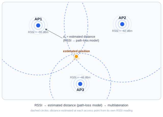
Every access point radiates its signal equally in all directions, and that signal weakens with distance in a predictable way. If a device knows an access point’s position and its transmitted power, and it measures how strong that signal is when it arrives, it can work out how far away it must be — the strength lost in transit is a function of distance alone. That gives one estimated distance per access point but, on its own, only narrows the device down to a circle (2D) or sphere (3D) around it, not a single point.
The trick is to do this for several access points at once. Each one narrows the possibilities down to its own circle; the position consistent with all of them is where those circles overlap — the same multilateration principle used by GPS. In practice, RSSI readings are noisy, so the circles rarely meet at one exact point: the estimator instead looks for the position with the smallest overall inconsistency across every reading, which is exactly what the linear, non-linear, and robust estimators below solve for, with increasing tolerance for noisy or wrong readings.
Path-loss distance model
Given a measured received power (dBm), a known transmitted power (dBm), a path-loss exponent , and signal frequency , the received-power model is:
where the frequency-dependent constant is:
( is the speed of light). Solving for the distance gives the conversion every RSSI estimator applies before running lateration:
Typical path-loss exponent values: free space , urban – , suburban – , indoor line-of-sight – . The non-linear and robust estimators additionally propagate the variance of , , and into a distance standard deviation via the first-order (delta method) derivative:
This conversion is implemented once, in Utils/PositionEstimatorHelper, and reused by every class below —
everything past this point is generic trilateration from (known position, estimated distance) pairs.
Class hierarchy
3D robust classes mirror the 2D ones (RANSACRobustRssiPositionEstimator3D, LMedSRobustRssiPositionEstimator3D,
etc.), omitted above for brevity. 2D estimators require a minimum of 3 sources; 3D estimators require 4 — one
extra source acts as the reference point that lets the trilateration equations be linearized.
The linear and non-linear indoor classes are thin wrappers that convert readings to
(position, distance, distance standard deviation) triples and then delegate to the generic lateration solvers
in the sibling com.irurueta.navigation.lateration package (irurueta-navigation module); the robust classes
delegate similarly to that package’s RobustLaterationSolver hierarchy.
Linear estimation
LinearRssiPositionEstimator picks one of two closed-form solvers (useHomogeneousLinearSolver, default
true) that both eliminate the path-loss model’s non-linearity by taking pairwise differences of the sphere/circle
equations before solving.
Inhomogeneous solver
Using the first source’s position as reference and letting be the estimated distance to source , subtracting the reference sphere equation from every other one cancels the quadratic terms in the unknown position, producing a linear system in the unknown offset :
solved by direct linear solve, then the reference position is added back. This is the default path for RSSI position estimation.
Homogeneous solver
Substituting homogeneous coordinates into the same pairwise-differenced equations produces a homogeneous system whose solution is the right null-space vector of (found via SVD); the estimated position is recovered by dividing by . It is more numerically robust to certain degenerate configurations, at the cost of an SVD instead of a direct solve.
Non-linear estimation
NonLinearRssiPositionEstimator minimizes, via Levenberg-Marquardt
(LevenbergMarquardtMultiDimensionFitter), the squared-distance residual between a candidate position
and each known source position , fit against the squared estimated
distance :
The initial position defaults to the centroid of the known source positions unless initialPosition is set
explicitly. Distance readings are weighted by their standard deviation (propagated from the path-loss model
above, or a fallback of ), and the fitter additionally reports a position covariance and
chi-squared value that the linear solvers cannot provide.
Robust estimation
RobustRssiPositionEstimator adds outlier tolerance on top of the linear/non-linear solvers, following the same
sample-and-score pattern for every variant:
The residual is always the trilateration distance error \(\left|\lVert \mathbf{p} - \mathbf{p}_i \rVert - d_i\right|\); what differs between variants is how candidates are scored and, for two of them, how samples are prioritized:
| Variant | Threshold semantics | Quality scores | Notes |
|---|---|---|---|
RANSAC |
Fixed |
not used |
Maximizes raw inlier count. |
MSAC |
Same |
not used |
Scores by truncated residual cost (residual capped at threshold) instead of a binary inlier count — a soft version of RANSAC. |
LMedS |
No inlier cut; minimizes the median of squared residuals. |
not used |
Robust even when the outlier ratio is unknown; typically needs more iterations. |
PROSAC |
Same |
required ( |
Samples higher-quality readings first instead of uniformly at random, converging faster when reading quality is known. |
PROMedS |
Same |
required, same as PROSAC |
LMedS’s median-residual robustness combined with PROSAC’s quality-guided sampling order. |
If isResultRefined (default true), the winning candidate is always re-solved with the non-linear solver
restricted to its inlier set, so every robust RSSI estimator ends up performing one final Levenberg-Marquardt pass
regardless of variant. The default robust method across the library is PROMedS.
Usage parameters
-
sources— located radio sources (RadioSourceLocated) with known position and transmitted power. -
fingerprint— theRssiFingerprintof readings observed at the unknown location. -
Linear:
useHomogeneousLinearSolver(defaulttrue). -
Non-linear:
initialPosition(else centroid),useRadioSourcePositionCovariance,fallbackDistanceStandardDeviation(default ). -
Robust (common):
confidence(default0.99),maxIterations(default5000),preliminarySubsetSize,isResultRefined(defaulttrue),isCovarianceKept(defaulttrue),evenlyDistributeReadings(defaulttrue, spreads sampling across sources so no single access point dominates). -
RANSAC / MSAC / PROSAC:
threshold(default ). -
LMedS / PROMedS:
stopThreshold(default ). -
PROSAC / PROMedS:
sourceQualityScores,fingerprintReadingsQualityScores(required).
Static create(…) factories on RobustRssiPositionEstimator2D/3D build any robust variant from a
RobustEstimatorMethod enum value.
API reference
Main classes used on this page, linked to their source code and Javadoc:
| Class | Source | Javadoc |
|---|---|---|
|
||
|
||
|
||
|
||
|
||
|
||
|
||
|
||
|
||
|
||
|
||
|
||
|
||
|
||
|
||
|
||
|
||
|
||
|
||
|
||
|
||
|
||
|
Related
-
Ranging-based position estimators — the equivalent hierarchy for distance (Wi-Fi RTT) readings.
-
Combined RSSI and ranging position estimators — estimators that combine RSSI and ranging readings.
-
Fingerprint-based position estimators — positioning without known source locations.
-
Radio source estimators — the inverse problem: estimating a radio source’s own position.