Gamma Function

This page was generated with the assistance of AI. Please report any inaccuracies.

The Gamma class implements the gamma function and the related functions built on top of it: factorials, binomial coefficients, the beta function, and the incomplete gamma function together with its inverse. The implementation follows the algorithms described in Chapter 6 ("Special Functions") of Numerical Recipes, 3rd Edition — see Reference for the full citation.

Gamma function and its logarithm

The gamma function extends the factorial to real and complex arguments and is defined by the integral

For a positive integer it reduces to the familiar factorial, offset by one, and it satisfies a simple recurrence relation:

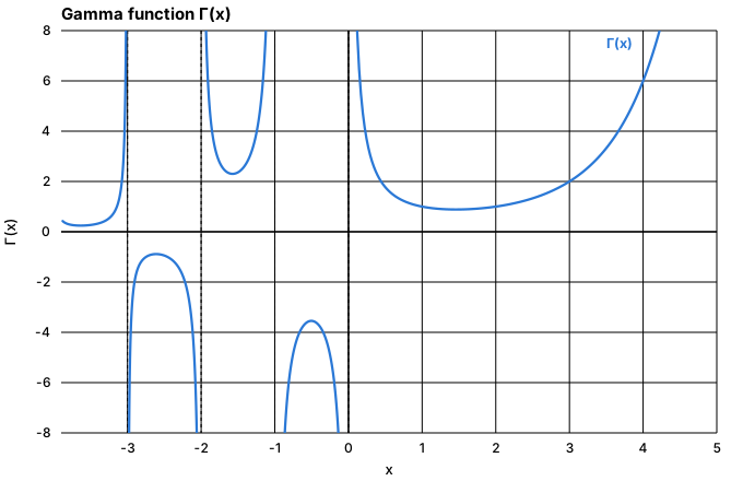
Plot of the gamma function showing poles at zero and the negative integers

Figure 1. Gamma function Γ(x). Poles occur at zero and every negative integer, where the function alternates sign between consecutive poles.

Because overflows for quite modest values of , the library follows the book’s recommendation and implements the logarithm of the gamma function, Gamma.gammln(xx), rather than the gamma function itself. gammln uses the Lanczos approximation, a rational-function approximation that is specific to the gamma function and accurate to better than over the whole positive real line:

with 14 precomputed coefficients (the COF array in the source code, taken from the coefficients calculated by P. Godfrey).

import com.irurueta.statistics.Gamma;

double logGammaOfFive = Gamma.gammln(5.0); // ln(4!) = ln(24)

Factorials and binomial coefficients

Because factorials are usually requested repeatedly for small integer arguments, Gamma.factrl(n) builds a lookup table of 0! to 170! on first use instead of calling gammln every time; 171! would overflow a double. Gamma.factln(n) similarly caches for n below 2000 and falls back to gammln(n + 1) beyond that. Both are used to compute the binomial coefficient

which Gamma.bico(n, k) evaluates from the factorial tables when n is small, and from factln differences (rounded with floor(0.5 + …) to clean up round-off error) for larger n.

double sixFactorial = Gamma.factrl(6);
double logOfLargeFactorial = Gamma.factln(5000);
double waysToChooseThree = Gamma.bico(10, 3);

Beta function

The beta function is defined by the Euler integral and relates to the gamma function as follows:

Gamma.beta(z, w) evaluates the right-hand side directly as a sum of logarithms, exp(gammln(z) + gammln(w) - gammln(z + w)), which avoids overflow for moderately large arguments.

double betaValue = Gamma.beta(2.0, 3.0);

Incomplete gamma function

The regularized incomplete gamma function and its complement are defined by

with the limiting values , , , and .

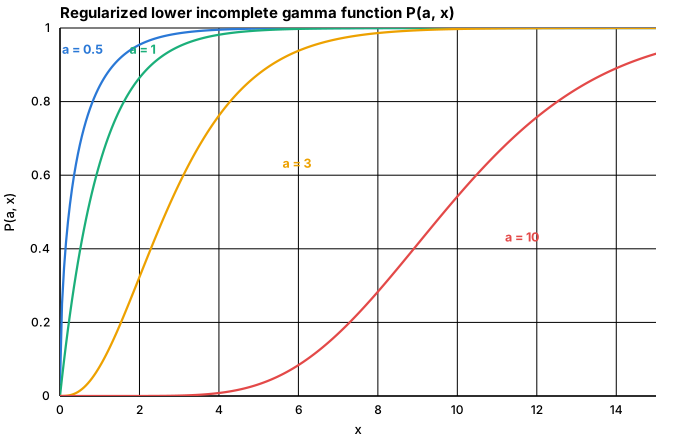
Figure 2. Regularized lower incomplete gamma function P(a,x) for four values of a. Small a rises to 1 almost immediately, while larger a delays the rise and flattens the curve into an S shape centered near x ≈ a.

No single numerical method is efficient across the whole plane, so Gamma.gammp and Gamma.gammq switch between three algorithms, exactly as struct Gamma does in the book:

A series expansion, which converges quickly for :
A continued fraction (its rapidly converging "even part"), used for :
A Gauss-Legendre quadrature of the defining integral, used once (the ASWITCH constant), where the series and the continued fraction both become inefficient. Gamma extends GaussLegendreQuadrature, which supplies the 18 abscissas and weights of the quadrature rule.

flowchart TD Start["gammp(a, x) / gammq(a, x)"] XZero{"x == 0?"} Large{"a >= 100 (ASWITCH)?"} NearA{"x < a + 1?"} Quadrature["Gauss-Legendre quadrature\n(gammpapprox)"] Series["Series expansion\n(gser)"] ContinuedFraction["Continued fraction\n(gcf)"] Start --> XZero XZero -- yes --> Trivial["P = 0, Q = 1"] XZero -- no --> Large Large -- yes --> Quadrature Large -- no --> NearA NearA -- yes --> Series NearA -- no --> ContinuedFraction

Both gser and gcf iterate until the relative change drops below machine precision, and throw MaxIterationsExceededException if that has not happened after 100 iterations — a situation the book notes as rare and limited to numerically unstable inputs.

import com.irurueta.statistics.Gamma;
import com.irurueta.statistics.MaxIterationsExceededException;

Gamma gamma = new Gamma();
try {
    double regularizedLowerIncompleteGamma = gamma.gammp(2.0, 3.0);
    double regularizedUpperIncompleteGamma = gamma.gammq(2.0, 3.0);
} catch (final MaxIterationsExceededException e) {
    // convergence was not reached for these inputs
}

Each call also updates gamma.getGln() with the value of used internally, in case a different normalization such as or is needed afterward.

Inverse incomplete gamma function

Gamma.invgammp(p, a) returns the value such that for a probability . It uses Halley’s method (a second-order variant of Newton’s method), which converges quickly because the derivative of with respect to is simply the gamma p.d.f. itself. A good initial guess is essential: for the implementation follows the normal-distribution-based approximation from Abramowitz & Stegun, and for it uses the book’s rough approximations

Twelve Halley iterations at most are then applied to refine this guess to full accuracy.

import com.irurueta.statistics.Gamma;
import com.irurueta.statistics.MaxIterationsExceededException;

Gamma gamma = new Gamma();
try {
    double xSuchThatPIsOneHalf = gamma.invgammp(0.5, 2.0);
} catch (final MaxIterationsExceededException e) {
    // convergence was not reached for these inputs
}

ChiSqDist uses gammp and invgammp directly to implement the chi-squared distribution — see Chi-Squared Distribution Algorithm. Erf computes the error function as a special case of the incomplete gamma function, although for performance it uses a dedicated Chebyshev approximation instead of calling Gamma at run time — see Error Function.