Lateration
| This documentation was generated with the assistance of AI. Please report any inaccuracies. |
The com.irurueta.navigation.lateration package recovers a position from a set of known reference positions and
their (possibly noisy, possibly outlier-contaminated) distances to an unknown point — the classic trilateration
problem, solved here for both 2D (intersecting circles) and 3D (intersecting spheres). Unlike
Frames and GNSS, this package is not based on
Groves, 2013; the linear solvers are based on
lemmingapex/trilateration and
Hereman & Murphy, as documented in the classes' own Javadoc and inline
derivations. See the bibliography for full citations.
What lateration is
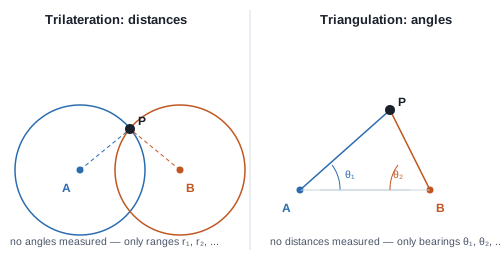
Lateration (trilateration when exactly three distances are used, multilateration when more are used) locates a point using only distance measurements to a set of known reference points — no angles involved. This is the key distinction from triangulation, which locates a point from angle (bearing) measurements taken at known points instead (Wikipedia, "Trilateration"; GIS Geography). GPS is the most familiar example: each satellite broadcasts its own position, the receiver measures its distance to each satellite (from radio signal travel time), and the receiver’s position is wherever those distances are simultaneously satisfied — no antenna pointing or angle sensing is involved.
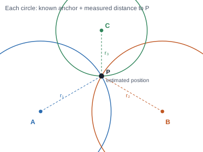
In the plane, a single distance measurement to a reference point A only constrains the unknown position to lie somewhere on a circle centered at A (all points a fixed distance from A). Two distances narrow this down to the (typically two) intersection points of two circles; a third distance to a non-collinear reference point resolves the remaining ambiguity down to a single point:
For a set of known 2D positions and their measured distances to the unknown point , the raw (unlinearized) system that lateration solves is simply "distance from the unknown point to each anchor equals the corresponding measurement":
and analogously in 3D, replacing circles with spheres and adding a coordinate:
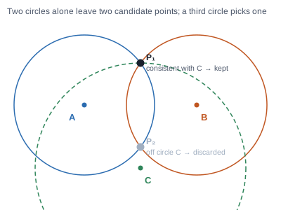
Each individual equation is nonlinear (quadratic) in the unknown position, and with exactly the minimum number of measurements (3 in 2D, 4 in 3D — one more than the number of dimensions, since one measurement is used as a reference when linearizing, see below) the system can have two solutions rather than one, unless the reference positions and the geometry rule one out:
In practice, measured distances are noisy (and occasionally wrong outright, e.g., a reflected or blocked signal), so real systems use more measurements than the strict minimum and fit the best position rather than solving the minimal system exactly — which is exactly what the rest of this page’s solver hierarchy does: linearize the system above to get a fast closed-form estimate (homogeneous and inhomogeneous solvers), optionally refine it against the true nonlinear equations (non-linear refinement), and optionally reject outlier measurements along the way (robust solvers).
Class hierarchy
There are two independent hierarchies rooted at Point<?> (2D Point2D or 3D Point3D): the non-robust
solvers, which assume every measurement is valid, and the robust solvers, which detect and discard outliers.
The robust hierarchy does not extend the non-robust one — it composes a homogeneous-linear, an
inhomogeneous-linear, and a non-linear solver internally and drives them from within its own estimation loop.
The same five robust variants (RANSAC, LMedS, MSAC, PROSAC, PROMedS) exist under RobustLateration3DSolver.
RobustLateration2DSolver.create(…)/RobustLateration3DSolver.create(…) are factory methods that dispatch
to the right subclass given a RobustEstimatorMethod.
Homogeneous linear solver
HomogeneousLinearLeastSquaresLaterationSolver linearizes the circle/sphere equations by treating the unknown
position as a homogeneous coordinate. For circles centered at with radius (the
known distances), subtracting the first circle’s equation from every other one cancels the quadratic
term:
Substituting the homogeneous coordinates turns this into a homogeneous linear system in (or in 3D), solved via the SVD of — the estimated position is the last column of , normalized by its component. At least 3 positions are required in 2D (4 in 3D).
var solver = new HomogeneousLinearLeastSquaresLateration2DSolver(positions, distances);
solver.solve();
Point2D estimatedPosition = solver.getEstimatedPosition();Inhomogeneous linear solver
InhomogeneousLinearLeastSquaresLaterationSolver instead picks the first position as a reference and subtracts
its equation from every other one directly in inhomogeneous coordinates. For positions :
giving a well-conditioned linear system with one fewer unknown than the homogeneous
formulation and no SVD needed — following
lemmingapex/trilateration and
Hereman & Murphy. This is the default preliminary solver used by the
robust hierarchy (RobustLaterationSolver.DEFAULT_USE_HOMOGENEOUS_LINEAR_SOLVER = false).
var solver = new InhomogeneousLinearLeastSquaresLateration2DSolver(positions, distances);
solver.solve();
Point2D estimatedPosition = solver.getEstimatedPosition();Non-linear refinement
NonLinearLeastSquaresLaterationSolver refines an initial position estimate (typically from one of the linear
solvers above) by minimizing the sum of squared residuals between measured and predicted distances using
Levenberg-Marquardt (LevenbergMarquardtMultiDimensionFitter). Because it fits the true nonlinear distance
function rather than a linearized version, it can also estimate the covariance of the resulting position and a
chi-square goodness-of-fit statistic.
var solver = new NonLinearLeastSquaresLateration2DSolver(positions, distances);
solver.setInitialPosition(coarseEstimate); // e.g., from the inhomogeneous linear solver
solver.solve();
Point2D refined = solver.getEstimatedPosition();
Matrix covariance = solver.getCovariance();Robust solvers
RobustLateration2DSolver/RobustLateration3DSolver handle measurements that may include outliers (e.g., a
non-line-of-sight ranging measurement). Internally, each maintains its own homogeneous-linear, inhomogeneous-
linear, and non-linear solver instances, and the robust estimation loop (RANSAC/LMedS/MSAC/PROSAC/PROMedS,
selected by subclass) drives them as follows for each random sample:
-
Solve the sampled subset with the linear solver (inhomogeneous by default,
DEFAULT_USE_HOMOGENEOUS_LINEAR_SOLVER = false) to get a coarse preliminary position. -
Optionally refine that preliminary position with the non-linear solver (
DEFAULT_REFINE_PRELIMINARY_SOLUTIONS = true). -
Once the robust estimator converges on an inlier set, optionally refine the final result again with the non-linear solver over just the inliers (
DEFAULT_REFINE_RESULT = true), optionally keeping its covariance (DEFAULT_KEEP_COVARIANCE = true).
| Method | When to prefer it |
|---|---|
|
Fast, general-purpose outlier rejection; good default when the inlier ratio is roughly known. |
|
No noise-threshold tuning required (uses the median residual); more sensitive to a very high outlier fraction. |
|
RANSAC variant with a smoother cost function; often converges with fewer iterations. |
|
Like RANSAC, but samples using a quality/prior ranking of the measurements, converging faster when such a ranking is available. |
|
LMedS with PROSAC-style prior-guided sampling. Library default
( |
var solver = RobustLateration2DSolver.create(
        positions, distances, RobustEstimatorMethod.PROMEDS);
solver.setConfidence(0.99);
solver.setMaxIterations(5000);
Point2D estimatedPosition = solver.solve();